Enhanced multi objective graph learning approach for optimizing traffic speed prediction on spatial and temporal features

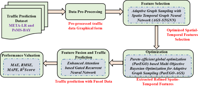
Experimental setup

The system specifications for this experiment include a hardware configuration of Intel Core i7-9700 K or AMD Ryzen 9 5900X processor, 64 GB DDR4 RAM or higher, 1 TB SSD storage or higher, and NVIDIA GeForce RTX 3080 or AMD Radeon RX 6800 XT graphics card. The software requirements include Windows 11 Operating system, virtual environment with conda, Python 3.8, tensorflow and Deep Graph Library (DGL) for graph construction package manager.

Dataset description

The performance of the proposed model is evaluated using two real-world traffic datasets METR-LA³⁷ and PeMS-BAY³⁸. METR-LA dataset consists of traffic data collected from 207 loop sensors across Los Angeles over the period of 4 months (March to June 2012) with 5 min of interval. It contains 1.5 million individual data points, covering speed, traffic volume, congestion levels, and timestamps. A crucial component of this dataset is the adjacency matrix (W_metrla.csv), a 207 × 207 weighted matrix representing connectivity between sensors. Each value in the matrix indicates a traffic-related metric, such as distance, congestion, or traffic flow strength, between sensor nodes. This matrix is vital for constructing the graph representation in the AGSTGNN model, capturing spatial dependencies among sensors. Their lies the unique sensor ID for each traffic sensor with the traffic congestion level categorised into low, high and medium. Also, the traffic data is observed in both the latitude and longitude time. The PeMS-BAY dataset contains 325 sensor stations considered for the period of 6 months with the features such as traffic speed, flow, and occupancy levels. Additionally, the dataset includes a metadata file (PEMS-BAY-META.csv), which provides details about freeway IDs, lane counts, location coordinates, and segment lengths. These features improve the proposed model’s generalization across diverse urban and highway environments.

Results and discussion

Evaluation metrics

The performance of the proposed model is evaluated using four metrics such as MAPE, MSE, MAE, RMSE, R² score are given in Eqs. (13)–(17). The following tables [Table] presents the equation for calculation, \({Y}_{i}\) – True samples, \({Y}^{v}\) – predicted values, \({Y}^{{v}_{i}}\) – mean value of \(Y\).

Model training and validation

Learning parameter setup

Adam Optimizer is utilised to tune the parameters such as learning rates, momentum and RMSprop for faster convergence in spatio temporal data. The model is trained with 100 epochs and data is split with the ratios 70:15:15. 70% samples are considered for training and 15% data is for testing. Similarly, 15% data is used for validation. The hyper parameter optimization using Bayesian optimization of pareto efficient global optimization was carried out at validation set, and the results are captured in the unseen test set. The following Table 1 captures the parameters utilised for the experimentation which ensures the model generalizes well and avoids overfitting issues.

The performance of the proposed model is evaluated with other baseline models by considering the two datasets in terms of RMSE, MAE and MAPE. Figure 4 represents the time-series plot of displaying the traffic speed in km/h for a period of 24 h. The cyclic pattern is followed for the traffic speed, it is observed that the traffic speed is increased for the 6–7 h, then it gets deteriorations considerably from 12 to 15 h. Finally, it rises to its peak at the end of the day. The grey line exposes the ground truth value, green line expresses the proposed model, orange and blue line represents the baseline models. It is observed that the proposed model tracks the ground truth value more closely whereas the baseline models exhibit fluctuations at peak hours. Also, it is observed that the proposed model performs better than the other models capturing the traffic speed dynamics with the spatial and temporal feature extraction patterns.

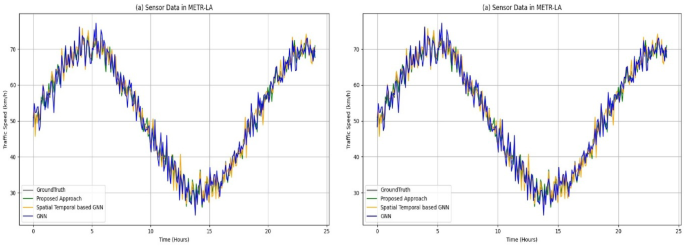
Time-Series Analysis on METR-LA and PeMS-BAY dataset using proposed vs. baseline methods.

From the below Fig. 5 it is observed that the proposed model captures the spatial and temporal patterns from the META-LR data efficiently. As left side diagram indicates that the traffic speed observed on Tuesday and Wednesday is little higher stating that the traffic is less on those days. In Saturday the vehicle speed is observed at 40 km/hr indicating that the traffic is higher than usual and again rises to 60 km/hr on Sundays which is indicates that reduced congestion in the traffic. The right-side diagrams specifies that the more fluctuations in the traffic speed from the time period of Jan till July, might relies on changes in the nature of the transportation. Adaptive graph sampling captures these fluctuations in the traffic speed by prioritizing the traffic time intervals in order to reflect the real time traffic/dynamic traffic patterns. Optimised MOBO approach ensured that the model is robust in traffic predictions. Also, the proposed model alleviates congestion traffic in this time. (a) Daily traffic speeds – The average vehicle speed is recorded in km/hr which is represented in blue line. The diagram is for each day of the week and the high-speed traffic observations are captured in red points. 4(b) Weekly Traffic Speeds – The blue markers indicate high-speed traffic observations on random dates between January and July, with a grey dashed line connecting them to highlight fluctuations. Our adaptive graph sampling (AGS) mechanism effectively captures these patterns, which are then optimized by MOBO to accurately reflect dynamic traffic trends.

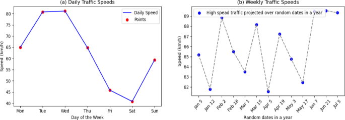
Spatial and temporal stamps of daily and weekly traffic speed.

Figures 6 and 7 illustrate the performance of the proposed model on META-LR and PeMS-BAY datasets, showcasing MAE and RMSE scores over 100 epochs. The MAE plot (Fig. 6) demonstrates a steady decrease in error, indicating improved prediction accuracy with training data, converging to ~ 2.10 and ~ 2.15 for META-LR and PeMS-BAY datasets, respectively. The RMSE plot (Fig. 7) also exhibits a decreasing trend, converging at ~ 3.29 for META-LR and ~ 3.21 for PeMS-BAY, highlighting the model’s robustness and generalizability. Both figures show minor fluctuations due to batch-level noise or learning rate dynamics, but no evidence of overfitting is observed, as the training curves converge smoothly without a “U-turn” pattern. The consistent decreasing trend in MAE and RMSE scores across epochs indicates continual learning and optimization of the model’s parameters, demonstrating its effectiveness in predicting traffic patterns.

MAE of META-LR Dataset and PeMs-BAY.

RMSE of META-LR and PeMS-BAY.

Figure 8 illustrate the validation performance of model on META-LR and PeMS-BAY datasets, showcasing MAE and RMSE over 100 training epochs. In Fig. 8, both datasets exhibit a downward trend with minor fluctuations, indicating steady improvement in prediction accuracy without sudden divergence. Similarly, Fig. 8, shows a slight decline followed by stabilization, suggesting effective learning and convergence. The performance trends indicate rapid decreases in MAE and RMSE during initial epochs, followed by stabilization after ~ 40–50 epochs, confirming convergence. Both validation MAE and RMSE remain stable, confirming retained generalization and posed a well-regularized training process. Overall, these plots demonstrate consistent performance improvement and no overfitting across both datasets.

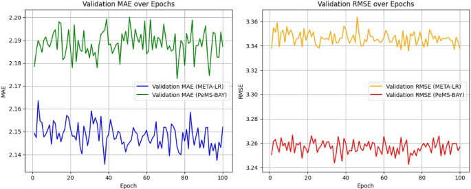
Validation of MAE and RMSE for META-LR and PeMS-BAY Datasets.

To ensure robust evaluation and prevent overfitting, we implemented a three-way data split strategy, dividing each dataset into 70% training, 15% validation, and 15% testing subsets. The training subset was used for learning model parameters, while the validation subset was exclusively used for hyperparameter tuning and early stopping. The testing subset was held out for final model performance evaluation, ensuring no data leakage. We conducted hyperparameter optimization using a Multi-Objective Bayesian Optimization (MOBO) framework.Table 2 captures the parametric values for the proposed model with the range explored and considered for training, validation Table 2.

To prevent overfitting, we used early stopping based on validation loss with a patience threshold, ensuring the model retains optimal generalization ability. This approach, combined with our rigorous training and evaluation pipeline, ensures reported performance metrics accurately reflect the model’s predictive capabilities on unseen data.

Figure 9 captures the MAPE comparison for the proposed model in the training data with two different datasets. MAPE values reduced from 3.20 to 3.17 over 100 epochs for training data, which increases the enhanced prediction percentage errors. For META-LR its has 3.17 value and for PeMS-BAY it achieved 3.21. Figure 10 captures the \({R}^{2}Score\) where it increase progressively from 0.75 to 1.00 epochs which echoes the strongest fitness between the actual values and the predicted values for the training data. Likewise, the values of \({R}^{2}Score\) increases from 0.75 to 0.95 for PeMS-BAY dataset indicates that the model exhibits the improved performance in Fig. 10.

MAPE for META-LR and PeMS-BAY.

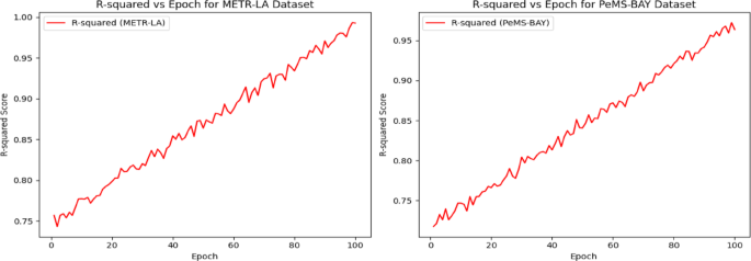
R squared score for METR-LA and PeMS-BAY.

Discussion

From the Table 3 it is inferred that the proposed model outperforms well on both the META-LR and PeMS-BAY dataset with lowest MAE (2.09), RMSE (3.29) and MAPE (3.17), similarly on PeMS-BAY dataset it has lowest values of MAE (2.15), RMSE (3.22) and MAPE (3.21). The existing DSTMAN³³ model on META-LR and PeMS-BAY had achieved MAE (2.94), RMSE (5.95) and MAPE(7.98) and the STGCN (Cheb)³⁴ have implemented in PeMSD7(M) and PeMSD7(L) which achieved MAE (2.25), RMSE(4.04) and MAPE(5.26) in PeMSD7(M) and the another dataset PEMSD(L) have MAE(2.37), RMSE(4.32) and MAPE(5.56).The STGCN³⁴ in PeMSD7(M) and PeMSD (L) have reached two different values, for PeMSD(M) had MAE (2.26), RMSE (4.07) and MAPE (5.24) and the PeMSD(L) have MAE(2.40), RMSE(4.38) and MAPE(5.63).Then, the GMAN³⁵ model in PeMS and Xiamen datasets have reached the MAE (1.86),RMSE(4.32) and MAPE(4.31) for PeMS dataset and the Xiamen dataset had achieved MAE(11.50), RMSE(12.02) and MAPE(12.79) and the final existing model BiGRU for the china peak MAE(22.08),RMSE(48.47),MAPE(9.67)and china low peak datasets have reached MAE(31.12),RMSE(10.19) and MAPE(24.61). Amongst all, Bi-GRU method shows higher errors when compared with all the methods. Apart from these observations, STGCN and GMAN methods exhibits better performance on the smaller datasets however, it is unknown about its performance on larger data. While proposed model shows better performance in all aspects, fortifying the robustness across different data ranges.

Comparison of MOGL approach with baseline models

The following Figs. 11 and 12 shows that by minimising prediction errors (MAE, RMSE) while decreasing percentage errors (MAPE), the proposed MOGL approach outperforms baseline models (GNN, GRU, LSTM, RNN) on both datasets. This demonstrates how well it works to solve issues like dynamic spatiotemporal interdependence and enhancing the precision of traffic speed predictions.

Figure 11 represents the MAE values for various models on META-LR and PeMS-BAY datasets. Amongst all models, the proposed model achieves the lowest MAE signposts its supremacy in prediction accuracy. RNN model exhibits highest MAE values for both the dataset indicating the poor performance over all the other models. LSTM, GRU and GMM performs better performance whereas not as better than the proposed model. The overall inference from this shows that the proposed model is effective in reducing the prediction errors by increasing the robustness of the model.

Comparison of MAE values for METR-LA and PeMS-BAY with existing DL models.

The Root Mean Square Error (RMSE) for each model on the META-LR and PeMS-BAY datasets is displayed in the Fig. 10. With the lowest RMSE (~ 3.29 for META-LR and ~ 3.22 for PeMS-BAY), the suggested model shows a smaller error magnitude. RNN has a large prediction deviation with the greatest RMSE (~ 7 for META-LR and ~ 5.5 for PeMS-BAY). Although GNN outperforms RNN, the Proposed Model still outperforms is show in Fig. 12. These outcomes demonstrate how well the Proposed Model reduces overall prediction errors.

Comparison of RMSE values for META-LR and PeMS-BAY with existing DL models.

The Mean Absolute Percentage Error (MAPE) of various models on the two datasets is shown in Fig. 13. With the lowest MAPE (~ 3.17 for META-LR and ~ 3.21 for PeMS-BAY), the Proposed Model exhibits the best percentage-based prediction accuracy. For both datasets, RNN has the highest MAPE (~ 9), indicating subpar relative error reduction performance. The Proposed Model outperforms LSTM, GRU, and GNN, which have modest performance. This attests to the Proposed Model’s dependability in lowering percentage mistakes.

Comparison of MAPE values of METR-LA and PeMs-BAY with existing DL models.

The \({R}^{2}\:Score\) for each model and dataset is shown in Fig. 14, which gives information about how well predictions match actual data. With the greatest \({R}^{2}\:Score\)of almost 0.92 for the METR-LA and PeMS-BAY datasets, the proposed model demonstrates a strong correlation between expected and actual results. On the other hand, the RNN model shows poor prediction dependability with a relatively low R2 Score of about 0.8. Although LSTM, GRU, and GNN models perform better than RNN, they are still not as accurate as the Proposed Model. The better performance of the proposed approach shows that it can produce forecasts that are more reliable and accurate. In applications where predicted accuracy is essential, this is especially important. The strong \({R}^{2}\:Score\) of the suggested model indicates that it can successfully identify the underlying relationships and patterns in the data. The other models’ lower \({R}^{2}\:Score\), in contrast, show a poorer relationship between expected and actual values. All things considered, the Proposed Model’s outstanding performance highlights its potential for practical uses.

Comparison of R squared score of METR-LA and PeMS-BAY with existing DL models.

The key findings from the above discussed subsections are the proposed model achieves lowest MAE value with 2.09 for METR-LA and 2.15 for PeMS-BAY model. This indicates that the efficiency of the proposed model with minimised prediction errors. This exceptional performance shows that the suggested model has effectively streamlined the learning procedure, producing precise predictions under a range of circumstances. Additionally, the performance of the model has been greatly improved by the use of multi-objective Bayesian optimization. The model has successfully navigated the intricate search space by utilizing this optimization strategy to find the ideal hyperparameters that reduce prediction errors. The result of this synergy between multi-objective Bayesian optimization and the suggested model is a strong and trustworthy forecasting framework. These results have significant ramifications, indicating that the suggested methodology can be successfully applied to real-world situations where precise forecasting is essential, such traffic flow prediction. The model’s potential for broad acceptance and use is shown by its strong generalization across various datasets and situations.

Comparison of imputation method

From the Table 4 it is observed that KNN achieved the lowest MSE and RMSE in both imputation and prediction which indicates that KNN suits well in all aspects. GRU-D suits for temporal gaps, slightly it underperformed which is possibly due to the limited number of data or overfitting in low level missing scenarios. Whereas, Linear Interpolation model was less effective in analysing the temporal patterns in complex data.

Ablation study

In Table 5, the baseline model was considered as gate recurrent unit (GRU ) without the feature selection process was implemented in two different dataset have greater values of MAE(25.4), RMSE(37.2) and MAPE(21.1). Then the graph-based pooling of STGNN with AGS was taken as feature selection technique have reached MAE(23.5), RMSE(34.2) and MAPE(18.9) better compared to simple GRU predict the traffic speed. Then, the Bayesian optimization based AGS is deployed as centrality-based sampling process have achieved MAE (21.5), RMSE (32.2) and MAPE (17.2). and the final is proposed approach MOGL have achieved (2.09) MAE, (3.29) RMSE and (3.17) MAPE has achieved stable performance with limited time complexity.

Comparison of proposed MOGL approach with statistical test

To validate the proposed MOGL approach robustness through 5 independent runs on META-LR and PeMS-BAY datasets, reporting mean and standard deviation for MAE, RMSE, MAPE, and R² Score in Table 6. The proposed model outperformed baselines with lower errors and higher R² scores. Paired t-tests confirmed statistically significant improvements (p < 0.05), demonstrating the model’s reliability for traffic speed forecasting under varying conditions.