An interpretable hybrid deep learning framework for gastric cancer diagnosis using histopathological imaging

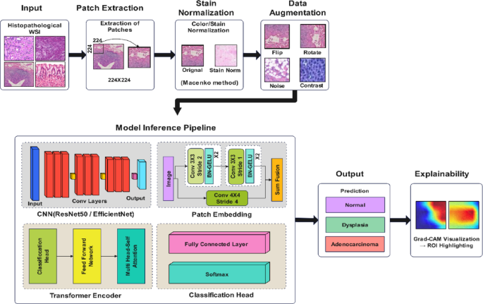
The proposed methodology is a five-stage pipeline that performs accurate and interpretable classification of gastric cancer from histopathological images. The system starts by extracting patches from whole slide images (WSI), followed by stain normalization to reduce color variability. A hybrid deep learning architecture is used, which takes input of augmented image patches and combines a CNN backbone (such as ResNet50 or EfficientNet) with a transformer encoder for global context modeling. To make the model robust, the model is trained with a cross-entropy loss function and stratified k-fold cross-validation. Finally, class-discriminating regions are interpreted using Grad-CAM for clinical validation. Figure 1 illustrates the proposed method’s complete workflow, from preprocessing to classification and interpretability, with both the architectural components and their clinical significance.

Proposed hybrid deep learning framework for gastric cancer classification and interpretability.

Datasets

This study utilizes three publicly available histopathological image datasets to improve model generalization and performance across diverse gastric cancer tissues. These datasets include GasHisSDB, TCGA-STAD, and NCT-CRC-HE-100 K. Together, they provide various image formats, staining protocols, and cancer subtypes, essential for training a robust and transferable classification model. The first dataset, GasHisSDB³⁶ is a dedicated gastric histopathology dataset developed by Guangdong Provincial People’s Hospital. It contains 245,196 image patches extracted from hematoxylin and eosin (H&E)-stained whole slide images. Each patch is sized at 160 × 160 pixels and categorized into three balanced classes: normal, dysplasia (pre-cancerous), and adenocarcinoma (cancerous). Expert pathologists curated and labeled these patches, making the dataset highly suitable for supervised deep learning applications in gastric tissue classification. The second dataset is derived from The Cancer Genome Atlas (TCGA)³⁷, specifically the Stomach Adenocarcinoma (TCGA-STAD) cohort. This dataset includes digital whole slide images (WSIs) of gastric tumors and adjacent normal tissues collected from over 500 patients. Due to the large image sizes and variability in resolution, all WSIs were processed through patch extraction. Patches of size 224 × 224 pixels were generated from clinically annotated tumor and normal regions for model training and external validation. The third dataset, NCT-CRC-HE-100 K 38, comprises 100,000 non-overlapping image patches of colorectal cancer tissue obtained from formalin-fixed, paraffin-embedded slides. Although it focuses on colorectal rather than gastric tissues, its inclusion in this study is a strong basis for transfer learning. The dataset comprises nine distinct tissue types, including tumor epithelium, stroma, and muscle, with all images uniformly sized at 224 × 224 pixels. The large scale and histological similarity between gastrointestinal tissue structures allow models pretrained on this dataset to adapt effectively to gastric cancer classification tasks. Table 2 present Summary of datasets used in this study. GasHisSDB serves as the primary dataset for training and evaluation, TCGA-STAD is used for external validation through patch extraction from WSIs, and NCT-CRC-HE-100 K supports pretraining via transfer learning across diverse tissue types.

These datasets were preprocessed consistently using stain normalization and quality filtering. Stratified sampling was applied to maintain class balance across training, validation, and testing sets. Each dataset was processed to ensure image normalization, labeling format, and patch resolution consistency. The combined use of domain-relevant gastric cancer data and related colorectal histology enables robust model development and supports transfer learning strategies to improve classification performance in resource-constrained or small-sample scenarios.

Preprocessing and augmentation

A standardized preprocessing pipeline was applied to all histopathological images to ensure consistency across datasets and improve model robustness. The first step involved resizing all image patches to a uniform resolution of 224 × 224 pixels. While GasHisSDB and NCT-CRC-HE-100 K already provide fixed-size patches, patches extracted from TCGA-STAD whole slide images were cropped to the same size to maintain compatibility during model training. Stain variability is a well-known challenge in histopathology due to differences in scanner types, staining protocols, and laboratory conditions. To address this, all images were normalized using the Macenko stain normalization method, which aligns color distributions while preserving tissue morphology. Training with this technique will minimize domain shift across multiple datasets and generalize well to unseen slides. During training, there was extensive data augmentation to increase dataset diversity and avoid overfitting. Augmentation techniques were horizontal and vertical flipping, random rotations (up to ± 30 degrees), brightness and contrast adjustments, and Gaussian noise injection. At runtime, these transformations were applied probabilistically using the Augmentations library, and so the model saw different visual variations in each training epoch. Specifically, for the TCGA-STAD dataset, background or artifact regions that exceeded the threshold value were excluded with an Otsu threshold tissue detection algorithm. Retained were only patches with sufficient tissue content to avoid noisy inputs affecting the model performance. In addition, all image intensities were zero mean and unit variance per channel before feeding them into the neural network. We propose the use of this preprocessing strategy, which standardizes input data and makes the model’s capacity to learn robust and transferable features between gastric and colorectal tissue domains.

Model architecture

The architecture proposed is a fusion of a Convolutional Neural Network (CNN) backbone with a Transformer encoder to make use of both local texture patterns and global contextual information of histopathological image patches. This hybrid technique has extended capability to overcome the weaknesses of traditional CNNs in identifying long-range spatial dependency, which is essential in identifying distributed malignancies in gastric tissue. Let \(X\in {\mathbb{R}}^{H\times W\times C}\) denote the input image patch of size \(H\times W\) with \(C\) color channels. The CNN backbone, denoted \({\phi }_{CNN}(\cdot )\), maps the input image to a lower-dimensional feature map:

where \(h\times w\) is the spatial resolution of the feature map, and \(d\) is the number of feature channels. In our implementation, we use ResNet50 and EfficientNet-B3 as backbone candidates, both pretrained on ImageNet and fine-tuned on our datasets. The CNN captures local patterns such as glandular structures, cellular arrangements, and tissue textures, which are essential for discriminating between normal, dysplastic, and malignant regions. To incorporate the Transformer, the feature map \(F\) is divided into non-overlapping patches. Each patch \({f}_{i}\in {\mathbb{R}}^{p\times p\times d}\) is flattened and projected into a lower-dimensional embedding space via a linear projection:

where \({W}_{p}\in {\mathbb{R}}^{D\times ({p}^{2}d)}\) is the learnable projection matrix, and \(D\) is the embedding dimension. A positional encoding \({PE}_{i}\)​ is added to preserve the spatial relationships between patches:

The full sequence \(Z=[{\widetilde{z}}_{1},{\widetilde{z}}_{2},\dots ,{\widetilde{z}}_{N}]\) is then passed to the Transformer encoder, where \(N\) is the number of patches. The Transformer encoder comprises multiple layers of multi-head self-attention (MHSA) and feed-forward networks (FFN). Each self-attention head computes:

where \(Q,K,V\in {\mathbb{R}}^{N\times {d}_{k}}\) are the query, key, and value matrices derived from the input \(Z\), and dk​ is the key dimension. Multi-head attention is defined as:

with each head computed independently using different projection matrices, allowing the model to jointly attend to information from different subspaces. Each Transformer block also includes layer normalization and residual connections:

The final output token \({Z}_{cls}^{{\prime}{\prime}}\)​ is passed through a multi-layer perceptron (MLP) classifier with a softmax activation:

where \(Wc\in {\mathbb{R}}^{K\times D}\) maps the encoded features to \(K\) output classes (e.g., normal, dysplasia, cancer), and \(\widehat{y}\)​ is the probability vector over classes. The model is trained using categorical cross-entropy loss:

where \({y}_{i}\)​ is the one-hot encoded true label. The overall architecture of the proposed hybrid model is illustrated in Fig. 2, where the CNN extracts spatial features and the Transformer enhances global attention across tissue regions.

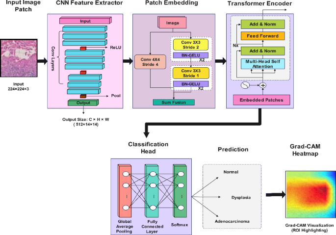
Proposed hybrid CNN-Transformer architecture.

The model was trained using a supervised learning framework. Input image patches were first passed through the hybrid CNN-Transformer architecture, which produced a probability distribution over the output classes. The model was trained end-to-end, with the CNN backbone initialized using pretrained weights from ImageNet and the Transformer layers initialized randomly. All images were resized to \(224\times 224\) pixels and normalized to have zero mean and unit variance across RGB channels. The complete inference process of the proposed hybrid CNN–Transformer model is outlined in Algorithm 1, which details each stage from input preprocessing to final classification and Grad-CAM-based explainability.

The dataset was split into training (70%), validation (15%), and testing (15%) subsets using stratified sampling to preserve class distribution. Data augmentation, including horizontal/vertical flipping, random rotation (\(\pm {30}^{\circ }\)), and brightness shifts, was applied on-the-fly during training to enhance generalization. Training was conducted for a maximum of 100 epochs with early stopping enabled based on validation loss. A mini-batch size of 32 was used. The model was trained on an NVIDIA A100 GPU, with each epoch taking approximately 2–3 min depending on architecture complexity. To reduce overfitting, dropout was applied with a rate of \(p=0.3\) after the Transformer encoder, batch normalization was used in the CNN layers, and L2 regularization was included in the optimization objective.

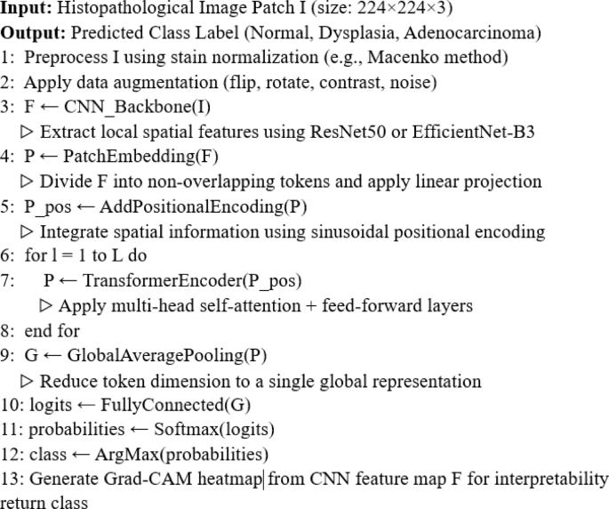
Algorithm 1: Hybrid CNN–Transformer Model for Gastric Cancer Classification.

Loss function and optimizer

We used the categorical cross-entropy loss function to optimize model parameters, suitable for multi-class classification. Let \({\widehat{y}}_{i}\) denote the predicted probability for class \(i\), and \({y}_{i}\in [\text{0,1}]\) the ground-truth one-hot label. The loss for a single input is given by:

where \(K\) is the number of output classes. The model aims to minimize this loss over the training dataset. To address mild class imbalance in some dataset subsets, we also experimented with weighted cross-entropy, where each class is assigned a weight \({w}_{i}\)​ inversely proportional to its frequency:

For optimization, we employed the Adam optimizer, which combines momentum and adaptive learning rates. The update rule for parameter \(\theta \) at time step \(t\) is:

where \({\widehat{m}}_{t}\) and \({\widehat{v}}_{t}\)​ are bias-corrected estimates of the first and second moments of the gradients, \(\alpha \) is the learning rate, and \(\epsilon \) is a small constant to prevent division by zero.

The initial learning rate was set to \(\alpha =1{0}^{-4}\), with a cosine annealing scheduler used to reduce it progressively over epochs. This approach balanced fast convergence and stability, particularly in deeper transformer-based models.

Evaluation metrics

To assess the performance of the proposed hybrid model, we employed several standard evaluation metrics for multi-class classification. These metrics capture various aspects of the model’s behavior, including correctness, sensitivity to minority classes, and overall discriminative ability. Accuracy is the proportion of correctly predicted samples over the total number of predictions:

In the multi-class setting, this becomes:

where \(N\) is the total number of test samples, \({\widehat{y}}_{i}\)​ is the predicted class, and \({y}_{i}\)​ is the true class label. For each class \(c\), we compute precision and recall as:

The F1-score for each class is the harmonic mean of precision and recall:

To summarize model performance over all classes, we use the macro-averaged F1-score:

where \(K\) is the number of output classes. Macro-averaging gives equal weight to each class, making it particularly informative in class-imbalanced settings. We also report a confusion matrix \(C\in {Z}^{K\times K}\), where \({C}_{i,j}\)​ indicates the number of samples with true label \(i\) predicted as class \(j\). This visualization provides insight into specific class-wise misclassification trends. This metric evaluates the model’s ranking ability and is robust to class imbalance. These metrics together provide a comprehensive evaluation of the model’s classification performance across multiple classes, balancing correctness, sensitivity, and interpretability.