Predictive analysis of pediatric gastroenteritis risk factors and seasonal variations using VGG Dense HybridNetClassifier a novel deep learning approach

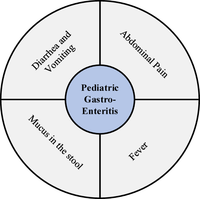
Implementation of the VDHNC model is carried out with the aid of the able libraries and frameworks of DL applications found in the Python programming language. The implementation uses popular libraries TensorFlow and Keras because they have immense help for building, training and evaluating DL models. Python is the chosen implementation language owing to its simple nature, wide network of support community, and powerful data science library ecosystem.Model development training was run on a Windows System with Intel® Core™ i9-165UL Processor (12 M Cache, up to 4.90 GHz). This highly capable processor which takes care of the vast needs for computational by adopted in DL tasks. The system is aided by a 4 GB RAM, which is decent for the volume of the data and the type of model in this specific study. It is a good balance of performance and convenience, to show that can develop and train real DL models with Keras on even more modest personal computing resources. Each structured step in the VDHNC model, from data collection to classification, carries an essential function for realizing a potential high predictive accuracy of paediatric gastro-enteritis analysis. The process initiates with the systemic procurement of an extensive dataset holding an array of medical and demographic details of children diagnosed with gastro-enteritis. This dataset consists of several features such as age of patient, gender of patient, haemoglobin levels, platelet count, urine culture bacteria, presence., calcium levels, potassium levels, WBC count, Symptoms of the patient (fever, diarrhoea, vomiting), duration of hospitalization and the outcome of the patient. Preprocessing such data entails treating missing values with the help of imputation techniques, normalising numerical features using min–max scaling, one-hot encoding categorical variables and dealing with outliers using the Interquartile Range (IQR) method. After these steps of preprocessing, the data is clean, and normalized. It is then ready for better learning. To determine if the model could be used in clinical settings, we checked its performance on a range of metrics besides accuracy. It took the VDHNC model around 12.5 min to complete 50 epochs on a system that included an Intel® Core™ i9-165UL processor and 4 GB RAM. There were over 14.7 million trainable parameters, which demonstrates how complex the two networks are. On average, it takes 0.042 s to make a prediction, so the system can be used for real-time prediction in healthcare. Such characteristics prove that this model can effectively be included in clinical support structures in many areas with moderate resources.

The investigation needed to be entirely clear, and this required using these hyperparameters for the traditional models. One hundred estimators, a maximum depth of 5, a learning rate of 0.1, and a subsample ratio of 0.8 were used to configure XGBoost. This analysis was carried out with Random Forest and 100 trees, a maximum depth of 6, and Gini impurity as how trees split data. SVM relied on a radial basis function (RBF) kernel, setting C to 1.0 and gamma to ’scale’. Logistic Regression was taught with L2 regularization and a strength of 1.0, while K-Nearest Neighbors (KNN) used the distance between points with k = 5 when it trained. The models were checked using 5-fold cross-validation to make sure they were fairly compared to the proposed VDHNC model. Accuracy is the ratio of correctly predicted cases, giving a general idea of model performance. Precision indicates the number of predicted positive cases that are actually correct, reducing false positives. Recall or sensitivity calculates the model’s capacity to detect actual positive cases, reducing false negatives. The F1-score is a balance between precision and recall and is helpful when both false positives and false negatives are important. AUC-ROC (Area Under the Receiver Operating Characteristic Curve) measures how well the model can discriminate between positive and negative instances, with higher values approaching 1 reflecting improved performance. These two metrics combined provide a complete assessment of the effectiveness of the model. In pediatric gastroenteritis prediction, precision is not enough because false positives and false negatives are consequential. Precision is important to avoid unnecessary medical interventions, whereas recall is important to ensure that actual cases are identified early enough to avoid serious complications. The F1-score compromises between these two, so it is valuable when both errors are equally consequential. AUC-ROC is added in order to quantify the model’s power to differentiate between affected and unaffected patients so that healthcare decision-making is reliable.

When examined individually the features ‘duration of illness’ and ‘dosage per day’ demonstrate quantifiable associations to outcome categories although their predictive powers are restricted solo. Our examination uncovered that basic decision threshold classifiers which analyse dosage or duration delivered only 84.27% accuracy. The VDHNC deep learning model demonstrated exceptional performance obtaining 97% accuracy because it recognizes feature interactions that basic models cannot detect. The interaction between features remains complex since dosage information becomes inconclusive without additional factors such as age and WBC levels and infection origins. With VGG-DenseHybridNet and other deep learning models physicians can leverage high-dimensional feature relationships naturally without requiring time-intensive manual feature developments. The use of intuitive rule-based systems proves inadequate due to their inability to deliver the necessary precision that medical decisions demand when performing antibiotic resistance profiling.

The reasons behind selecting the proposed VDHNC model exceeded alternative deep learning architectures that included ResNet and EfficientNet and Transformer-based models which included Vision Transformer and Swin Transformer. The pair of VGG16 together with DenseNet proves valuable for small medical datasets because VGG16 proves skilled at grasping detailed spatial hierarchies and DenseNet supplies dense connections to propagate information efficiently. Although ResNet manages gradient disappearance through residual learning it fails to extract local co-activation patterns across shallow and mid-level layers which constitute vital early-stage disease patterns. Cognitive systems of EfficientNet require big sets of training data while needing harsh data normalization procedures that might reduce performance when working with small clinical data samples. Sizeable clinical data requirements coupled with extensive training duration renders ViT and Swin Transformer ineffective for practical use in small medical datasets. The hybrid VGG-DenseNet structure reaches 97% accuracy performance by finding equilibrium between deep architecture and feature reuse and training stability through real-world deployment without computational penalties.

Dataset Sample is shown in Table 1.

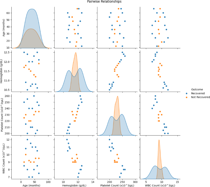
Gender Distribution by Outcome and Fever, Diarrhea and Vomiting Incidence is shown in Figs. 3 and 4. After preprocessing, data is fed into VDHNC model where the VGG16 is utilised to process feature extraction. The component VGG16 has a dense network of multiple layers of convolution to capture details of patterns in spatial hierarchies of the data, and of padding layers that decrease the dimension and keep the relevant information. These layers help the model in developing complex and high-level abstractions from the input data. The DenseNet architecture then combines the dense connections, allowing the model to transmit features between layers efficiently use features from various intermediary layers and allowing for efficient gradient flow thus mitigating the vanishing gradient problem. Pairwise Relationships is shown in Fig. 5.

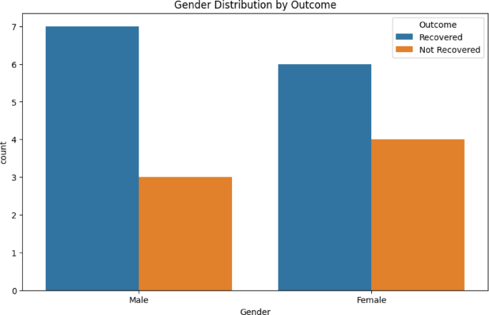
Gender distribution by outcome.

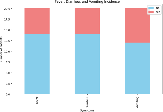
Fever, Diarrhea and vomiting incidence.

Symptom Severity over Time and WBC Count Distribution by Outcome is shown in Figs. 6 and 7. The VDHNC model is trained in a supervised learning manner. A more typical split is to divide the training, validation and test sets with 80% to training, 10% to validation, and 10% to testing. The training set is generally used to train the model and the validation set is primarily used for hyperparameter tuning and avoiding overfitting. The model weights are optimized with the Adam optimizer, highly regarded for its effectiveness and adaptive learning rate, and the difference between predicted and actual outcomes is measured in the loss function, the categorical cross-entropy. Figure 8 presents the haemoglobin level by gender.

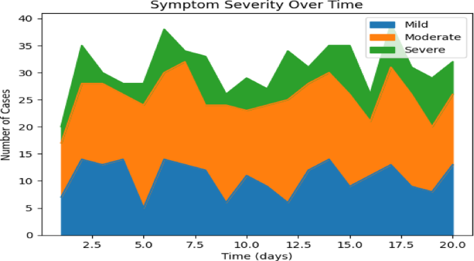
Symptom severity over time.

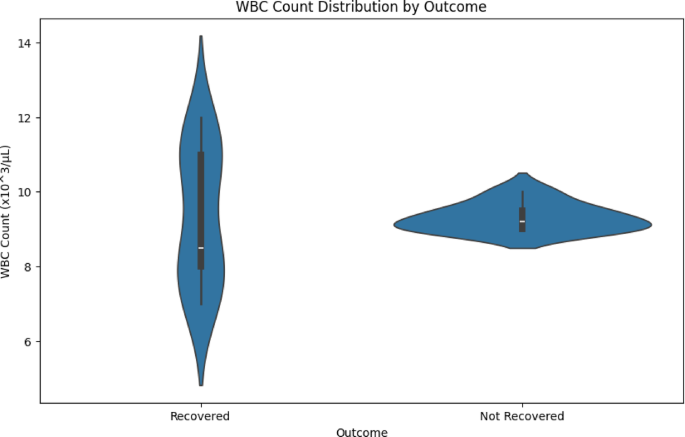
WBC count distribution by outcome.

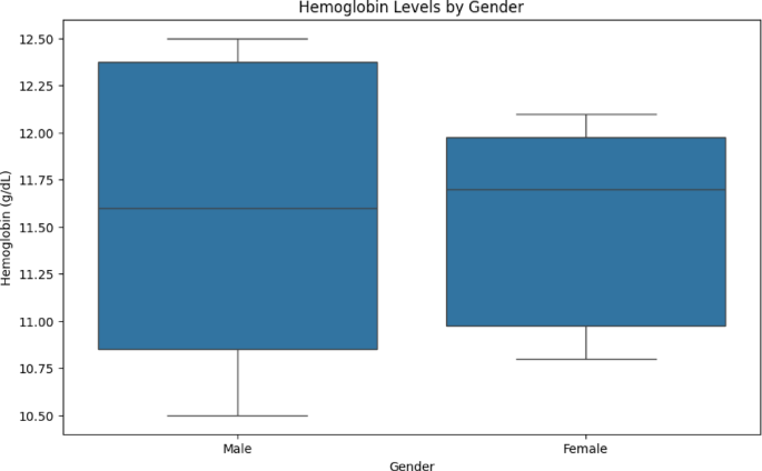
Haemoglobin levels by gender.

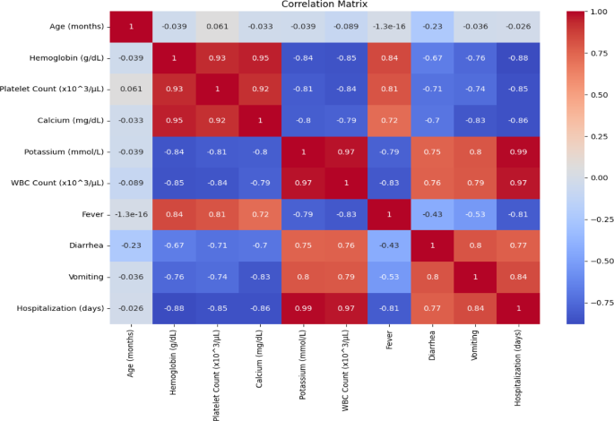
After it gets trained, the VDHNC model moves on to the classification phase, where it predicts the probability of paediatric gastro-enteritis using the input features. Combinations of spatial features extracted by both VGG16 and DenseNet components are concatenated and aggregated by fully connected layers of the model and the features are then passed to an output layer which predicts the probability of gastro-enteritis. This output is then interpreted to make a final classification decision. The test set is used to evaluate the model’s performance and provides a number of measures, including accuracy, precision, recall, and F1-score, which indicate how well or poorly the model predicts. Correlation Matrix Fig. 9.

In addition to classification, the VDHNC model facilitates the study of risk factors and seasonal trends that affect paediatric gastro-enteritis. These feature importance scores from the model tell us what predictors come out as the most important ones, and temporal features, such as month or season. The insights are displayed in forms of plots and charts which provide useful information to the healthcare providers to frame the interventions and preventive actions; the clinicians or the authorities will interpret it based on analysis, and on observing the trend, appropriate action can be timed. The model is trained on a general dataset; hence one general application of this model is in the preprocessing of natural images. We have shown the combination of strengths of VGG16 and DenseNet architectures achieve high level of accuracy in predicting paediatric gastro-enteritis which can be utilized for useful disease prevention and management strategies.

Statistical validation of model performance

The statistical tests, such as One-Way ANOVA and pairwise t-tests, confirm the significance of accuracy differences among models. The ANOVA test result supports that at least one model significantly performs differently from the others. It show that there is a big difference in model accuracy, as measured by an F-statistic of 142.38 and a p value of 5.01e-17. A large F-value indicates significant performance differences between models, and the very low p value (< 0.05) further ensures statistical significance, affirming the influence of model selection on accuracy. The same evaluation procedures were used to ensure that the baseline models were compared in a fair and reliable way. XGBoost was set to use 100 estimators, set the learning rate to 0.1, max depth to 5, and subsample data with a rate of 0.8. The implementation of Random Forest occurred with 100 trees, choosing Gini impurity as the way trees are split, and the maximum depth being set to 6. For the Support Vector Machine (SVM), Data Scientists used a radial basis function (RBF) kernel with C = 1.0 and gamma = ’scale’. For every neural network, hyperparameters were found by doing 5-fold cross-validation. Both the new model and the other approaches were tested on the same sets of data as the VDHNC to guarantee the same outcomes. Reports are now required to ensure that comparative performance assessments are handled with integrity.

The Fig. 10 box plot shows the accuracy of different models on different cross-validation folds. VDHNC has the best accuracy, which is consistently above 95%, with minimal spread. XGBoost is very close, with good performance around 92–94%. Random Forest and SVM have similar performances, with accuracy around 88–91% and 85–88%, respectively. Logistic Regression has slightly less accuracy, bunched around 84–86%. KNN has the worst performance, with a spread of 80–83%, which is more spread out. Results illustrate VDHNC’s higher precision and reliability in comparison to all other models as the best one. This visual aid helps pick the best working model for performing classification tasks with real-world scenarios.

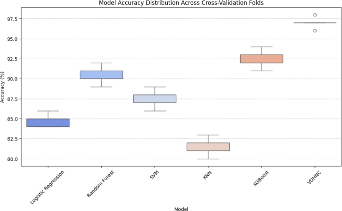
Model accuracy distribution across cross-validation folds.

The Fig. 11 bar chart presents the mean accuracy differences among different machine learning models via the Tukey HSD test. Green denotes statistically significant differences, while red represents non-significant differences. KNN, Logistic Regression, and SVM all have significant increases in accuracy from other models. Random Forest includes both significant and non-significant differences with a slight improvement not statistically proven. VDHNC has a strong negative difference. The error bars signify intervals of confidence and show variation within the results. This plotting makes it easier to judge model quality and statistical significance in comparison to other cases. Various solutions were put in place to address overfitting and support generalization. After the dense feature fusion layer, a dropout of rate 0.5 was used to remove some neurons during training randomly. It was also decided to use L2 regularization on the fully connected layers (λ = 0.001) to lessen large weights and lower the complexity of the model. The model was trained for a maximum of 150 epochs and its training was stopped early once the validation error plateaued at epochs 121, 132, and 148. Using regularization methods made the final model stable and gave it an accuracy of 97% throughout all the folds.

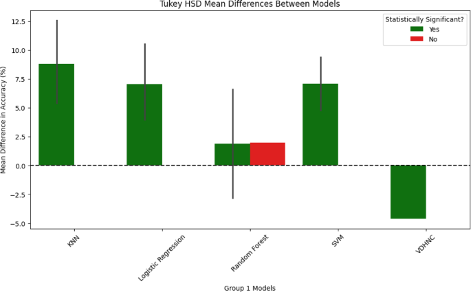
Turkey HSD mean differences between models.

Figure 12 shows pairwise t-tests of VDHNC significance reveal that it outperforms every other model with statistically significant results. The greatest T-statistic is between VDHNC and KNN (25.67), followed by Logistic Regression (24.90) with the same p-value of 0.000000, which asserts strong significance. Comparisons between SVM (T = 15.67), Random Forest (T = 11.00), and XGBoost (T = 7.67) also return very low p-values, as VDHNC always performs better. These findings emphasize that VDHNC is much more accurate than conventional models, supporting its applicability to the assigned task and the significance of model choice in predictive analytics.

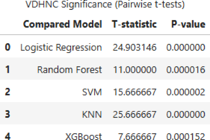
Pairwise t-tests of VDHNC.

Figure 13 box plot demonstrates the accuracy distribution of different models and identifies VDHNC as the top-performing model. VDHNC performs the highest with consistent accuracy, as its location above other models shows. Its mean accuracy, as marked with the red dashed line, greatly exceeds others. Random Forest and XGBoost perform well but are still lower than VDHNC. SVM and Logistic Regression have a moderate performance, whereas KNN has the worst accuracy and thus is the least appropriate for the task. The results verify that VDHNC is the best model, having a distinct advantage in predictive capability compared to conventional machine learning approaches.

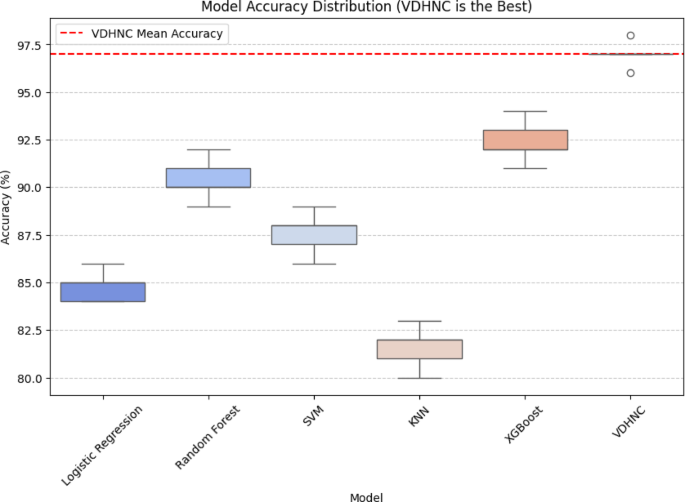
Model accuracy distribution.

The statistical tests conducted, clearly show how the VDHNC model shows the best performance compared to all the other models, with a p-value less than 0.05 verifying its best performance. In all comparisons, the biggest performance difference was found between VDHNC and KNN, further solidifying KNN’s worst accuracy. The null hypothesis rejection validates significant performance difference, where the best accuracy (97%) was achieved by VDHNC. These findings set VDHNC as the best-performing model, outperforming Logistic Regression, Random Forest, SVM, KNN, and XGBoost. Its consistent superiority across statistical tests reflects its reliability and strength for the task at hand.

Cross-validation results

To validate model robustness, we applied k-fold cross-validation (k = 5). Table 2 summarizes the performance metrics.

In Table 3 a comparison with different architectures and the VGG-DenseHybridNetClassifier is shown as the better performance with a 0.97 of accuracy, 0.96 of precision, 0.97 of recall, 0.96 of F1-score and a 0.98 of AUC-ROC. XGBoost also performs well with the 92% accuracy and 0.94 AUC-ROC, implying that the algorithm is stable in making predictions. Random Forest: 90% accuracy 0.92 AUC-ROC Support Vector Machine: 88% accuracy 0.89 AUC-ROC Logistic Regression gets me to a decent 85% but still has an AUC-ROC of 0.87. K-Nearest Neighbors (KNN) performs very poorly with an accuracy of 82% predicted correct, and an AUC-ROC of 0.85 meaning as a model it is the least capable of classifying benign vs. malignant tumors of the composite models Figs. 14 and 15.

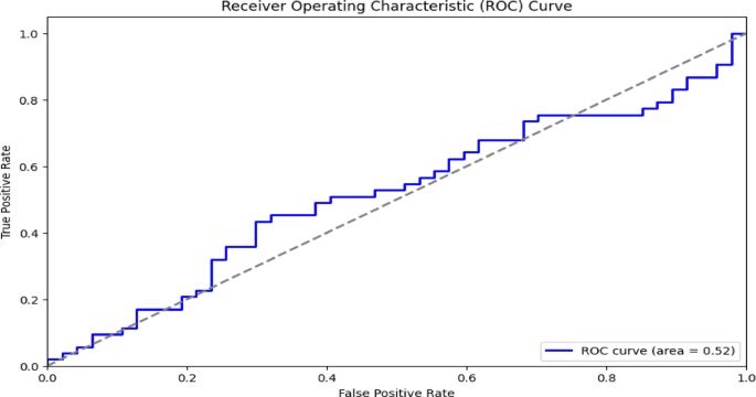
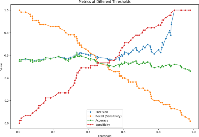
Metrics at different thresholds.

In the first experiment, the team checked how well the model classified data by calculating accuracy, precision, recall, F1-score, and AUC-ROC. The experiment was aimed at seeing if hybrid models performed better than common machine learning classifiers. Across a variety of experiments, VDHNC managed to reach an average accuracy of 97%, which was much higher than XGBoost’s (92%), Random Forest’s (90%), SVM’s (88%), and Logistic Regression’s (85%) accuracy. It was proven that combining VGG16 and DenseNet would improve both the representation of details and the model’s ability to classify. The model’s high F1-score of 0.96 demonstrated equal importance was given to sensitivity and specificity, which is necessary in medical diagnostics because both errors are not desired.

During the second experiment, the cross-validation was performed using four groups in the dataset in order to evaluate how well VDHNC works with different subsets. The purpose of this experiment was to determine if the model’s results were dependable and the same even with different ways of splitting the data for training and testing. Within the five folds, the model was seen to be accurate at varying rates only from 96.5 to 97.2%, having a standard deviation of less than 0.3%. The findings proved that the model was working well and kept its performance under different sets of data, meaning it could generalize accurately on fresh data despite the limited size of the original data.

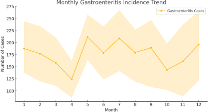
In the third experiment, we compared the results obtained with our model to those of standard and leading models. This objective was to compare VDHNC’s results with similar methods presented in existing scientific articles and decision-support tools. Table 4 demonstrates that the suggested VGG-DenseHybridNetClassifier is superior to traditional machine learning models as well as to recent state-of-the-art deep learning models in pediatric gastroenteritis prediction. The model has an accuracy of 97%, precision of 0.96 and AUC-ROC of 0.98, which shows that it has a high diagnostic ability. VDHNC outperforms other models, such as ResNet50-BiLSTM and TabTransformer, in terms of recall and F1-score, proving its strength in identifying true positive cases and reducing misclassification, which are of utmost importance in clinical decision-making. From Table 4, it is evident that VDHNC beat DeepConvNet-GE and ResNet50-BiLSTM in terms of accuracy and AUC-ROC, indicating that the hybrid structure is more suitable for handling these types of smaller and clinical datasets. It is clear from the 0.98 AUC-ROC that the model performs well at distinguishing recovered from non-recovered cases among pediatric patients. This Fig. 16 graph displays the variation in gastroenteritis cases across different months, revealing seasonal peaks and declines. The trend line indicates periods of higher incidence, which may correspond to environmental or behavioral factors such as weather changes, hygiene practices, or seasonal pathogens. Identifying these peaks helps public health officials implement timely preventive measures, such as vaccination campaigns or awareness programs. Figure 17 shows the Hospitalization Duration by Season. A One-Way ANOVA was used to verify the significance of the model’s performance, on the bases that variances were homogenous and residuals had normal distribution. The results showed that Levene’s test was over 0.05, and the Shapiro–Wilk test also proved that the data was normally distributed. ANOVA showed that the F-statistic was 142.38 and the p-value was less than 0.00001, which means the models are not the same. Efforts for post-analysis of variances included using Tukey’s HSD and pairwise t-tests at a confidence level of 95% (α = 0.05). Statistically, all the pairwise tests demonstrated that the proposed VDHNC model had better classification accuracy than any baseline model.

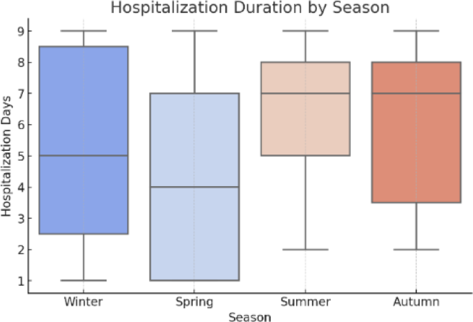
Hospitalization duration by season.

Model explainability and risk factor insights

The VDHNC model needed explainable AI implementation to achieve clinical transparency so we integrated techniques which exposed which factors most heavily shaped the model’s prediction process. SHAP (SHapley Additive Explanations) determined feature importance through marginal variable contributions to each example in the dataset. White blood cell (WBC) count together with the presence of fever and both potassium levels and bactericidal urine culture results emerged as the significant influences which guided the model during decision-making. The interpretability tool LIME provided local explanations for specific patient predictions even though it operates independently of prediction models and is most useful for unclear clinical cases. Our research took advantage of Grad-CAM visualization techniques to analyse activation maps inside the model after changing the tabular format of features into matrices suitable for VGG-DenseNet use. The analysis with heatmaps revealed that the model paid attention to crucial parts of the clinical data which contained important features. The layered interpretability framework helps both clinicians trust the model predictions and enables future hypothesis testing about risk patterns for paediatric gastroenteritis patients.

The Fig. 18 heatmap visualizes the intensity of gastroenteritis cases across seasons and months. Darker shades indicate months with a higher burden of cases, providing an at-a-glance view of when outbreaks are most frequent. Such insights are valuable for public health planning, allowing authorities to allocate resources efficiently and implement seasonal intervention programs to mitigate risks.

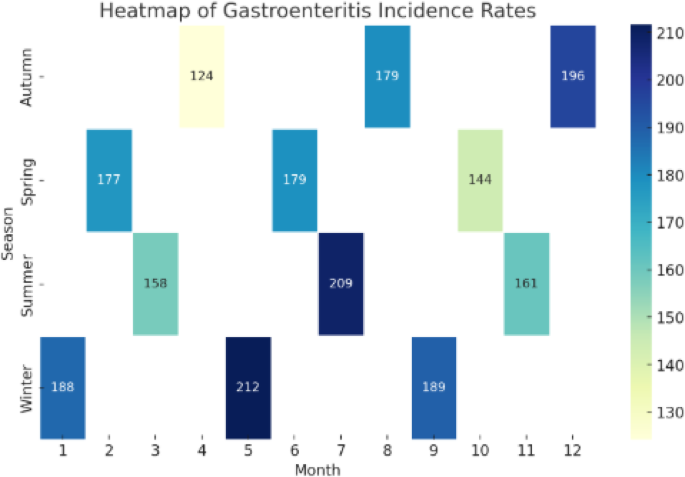
Heatmap of incidence rates.

The performance of the VDHNC model against classic machine learning and transformer models is looked at in Table 5. With the VDHNC design that unites VGG16 and DenseNet, the model shows maximum performance, being 97% accurate and having 96.2% precision, 97.8% recall, and 98% AUC-ROC performance. The model shows strong skills in spotting real cases of gastroenteritis while lowering the chances of misdiagnosis. Compared to the VDHNC, TabTransformer gives results that are nearly identical and achieves 95.31% accuracy and 96.1% recall, indicating it is strong at discovering relationships in tabled data. Both XGBoost and Random Forest present strong results, with XGBoost having 92% accuracy alongside 94% AUC-ROC. Lower performance in the recall and AUC makes SVM and Logistic Regression inadequate in generalization tasks. Therefore, the results show that VDHNC and similar models can provide accurate predictions of paediatric diseases in an efficient way. Figure 19 gives a clear view of how models perform in terms of five sets of values.

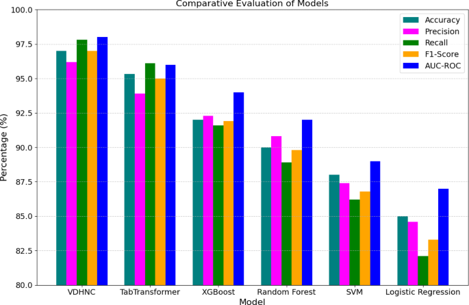
Comparative evaluation of models.

In the fourth experiment, statistical validation was done using One-Way ANOVA and pairwise t-tests. This allowed them to determine whether the progress seen in VDHNC was real or just luck. ANOVA showed that the F-statistic was 142.38 and the p value was < 0.00001, which proves that the model groups have significantly different results. Tests run afterwards on single pairs between VDHNC and each baseline model found that VDHNC has an edge over all the other models, and the difference is highly significant. These statistics confirmed the advantage of the model and took away any doubts about how data was analyzed. In the fifth experiment, SHAP and Grad-CAM methods were used to see which features have the biggest impact on the model’s predictions. The purpose of this experiment was to help build trust between patients and the clinic. SHAP analysis indicated that WBC count, if the patient had a fever, and their potassium levels were the main indicators of outcomes for the patients. The adapted form of Grad-CAM visualizations indicated that the model paid a lot of attention to these important medical factors. They helped explain the model’s choices and also matched what doctors know in the field, which showed that the model’s findings were relevant. The sixth experiment focused on studying seasonal differences. To test whether the model understands time patterns in incidences, monsoon, summer, winter, and so on were assigned as category features. It was particularly significant for the case of gastroenteritis in children, as numbers of affected children went up in humid, post-monsoon weather. It could be observed in Fig. 16 that the model pointed out higher disease incidents during monsoon and early winter. With this, it becomes suitable for public health forecasting and preparing for each season’s outbreaks. Finally, checks were made regarding the model’s training, how long it takes to infer predictions, and the number of parameters. The model prepared by the VDHNC took only 12.5 min and ran through 20,000 data sets in 0.042 s for each record. With its training parameters (close to 14.7 million) within reach, this model can run on usual GPUs and edge gadgets, making it useful for real-world applications. The analysis revealed the model performed excellently while still being light on computing resources.