Prediction of stillbirth using machine learning methods

Data source

Data were extracted from a perinatal database for women who delivered between January 2009 and December 2020 at seven hospitals in four areas of South Korea under the authority of The Catholic University of Korea. Data of maternal demographic characteristics, BMI, blood pressure (BP) measurements, blood and urine laboratory tests, diagnoses recorded by physicians, and medications prescribed were collected from the hospitals’ databases via electronic medical records (EMR). These data source were similar as the previous study¹⁹. This study was approved by the Institutional Review Board of the Catholic University Medical Centers (XC20WIDI0103). All methods were performed in accordance with the relevant guidelines and regulations. Informed consent was waived due to its retrospective study design.

Definitions of stillbirth

Stillbirth was defined as a baby born without signs of life after a threshold 20 weeks of gestation¹. International Classification of Diseases-10 (ICD10) code of O36.4 was used to extract the stillbirth group from the EMR. Early stillbirth was defined as stillbirth between 20^+ 0 weeks and 27^+ 6 weeks of gestation and late stillbirth was defined as stillbirth after a threshold 28 weeks of gestation²⁰. Multiple pregnancy, maternal age less than 18 years old at delivery, delivery before 20 weeks of gestation, and pregnancy with fetal chromosomal abnormality were excluded to ensure the homogeneity of the study population and reduce confounding factors that could affect the prediction models. Data were confirmed and missing data were abstracted from chart reviews by two obstetricians (J.H.W. and H.S.K.).

Machine learning analysis

Data preparation

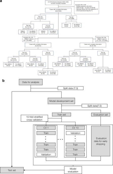
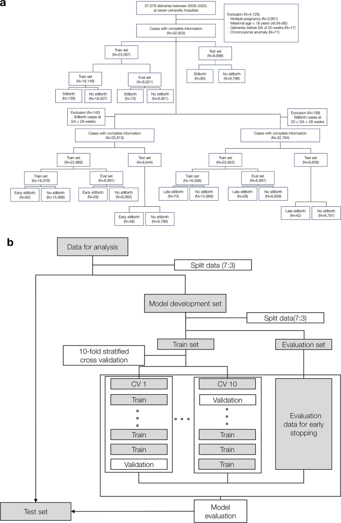
We followed guidelines for Transparent Reporting of a Multivariable Prediction Model for Individual Prognosis or Diagnosis for Establishing Prediction models²¹. Based on these guidelines, all anonymized data from 32,953 subjects were included in the data set used for this study. Subjects were assigned into two groups based on their parity status: nulliparity (n = 17,042) and multiparity (n = 15,911). To ensure a balanced distribution of target variable, a 7:3 stratified split was performed to divide data into training and test sets for each of the three cohorts²²: the whole cohort, the nulliparity cohort, and the multiparity cohort. Each cohort of training and test data was analyzed by dividing it into stillbirth and non-stillbirth groups. Because dataset was separated by birth, mothers with multiple births are shared between the training and testing sets.

Variables used to develop stillbirth prediction models

Three sets of variables were used to develop stillbirth prediction models, including variables from different time periods: (1) baseline variables obtained solely from maternal questionnaires completed during the first hospital visits, (2) 1st trimester (E1) variables collected until 13 weeks of gestation, (3) early third trimester (T0) variables collected until 28 weeks of gestation. For predicting all stillbirths and early stillbirths, baseline and E1 variables were used. For predicting late stillbirths, T0 variables were also used. These variables included age, parity, underlying diseases, family history, reproductive history, physical examinations, laboratory results, and obstetric histories of the previous pregnancy for parous women. All sets included age, parity, underlying diseases, reproductive history, obstetric histories of the previous pregnancy, physical examination, and family history. The baseline set included 123 variables for nulliparous women and 145 variables for parous women. The E1 set included variables at baseline and laboratory and ultrasonographic results until E1, which were 175 variables for nulliparous women and 197 variables for parous women. The T0 set included 410 variables for nulliparous women and 432 variables for parous women. The whole cohort used the same sets of variables as those used for the multiparity cohort according to each time point.

Machine learning algorithm and interpretation

XGBoost is a tree-based algorithm that operates based on the Gradient Boosting technique²³. In this study, extreme gradient boosting machine (XGBM) algorithm with built-in method for handling missing values was used, making it possible to use data with missing values in the machine learning process²⁴. We further enhanced our model’s performance by employing Optuna for systematic hyperparameter tuning, identifying the optimal settings to maximize predictive accuracy. Optuna is a tool designed for selecting machine learning models or determining hyperparameters, specializing in simplifying and streamlining the optimization process²⁵. Feature selection and hyperparameter tuning were performed using Grid Search with 10-fold cross-validation within the training set (Fig. 1b). An evaluation set was further separated from the training data and used exclusively for early stopping to prevent overfitting. To further address overfitting issues, we reduced the number of early stopping rounds to 10 and adjusted key hyperparameters. The adjusted hyperparameters include n_estimators, colsample_bytree, gamma, learning_rate, max_depth, min_child_weight, random_state, scale_pos_weight, and subsample. These changes were made to enhance the model’s generalization and reduce the performance gap between the training and test sets. The split data set was fed into algorithm and its performance was evaluated using metrics of area under the receiver operating characteristic curve (AUC), area under precision-recall curve (AUPR), specificity, F1 score, precision, and recall.

(a) Participants flow chart. GA gestational age, (b) Machine learning flow chart. CV cross validation.

Confidence intervals (CIs) for these metrics were calculated using a normal approximation based on the assumption of a binomial distribution. The z-value corresponding to the desired confidence level, such as 1.96 for a 95% confidence interval, varies depending on the confidence level and was computed using the scipy.stats.norm.ppf function. The length of the confidence interval (CI length) was then calculated using the following equation: CI length = z * √[m(1 – m) / n], where m is the calculated metric, n is the sample size, and z is the z-value corresponding to the confidence level. Finally, the lower and upper bounds of the confidence interval were determined by subtracting and adding the CI length from the metric value: CI lower bound = m – CI length, CI upper bound = m + CI length.

This approach ensures that the confidence intervals are accurately calculated using the binomial distribution assumption. Shapley values were used to indicate how much influence each variable had in determining model output. The Shapley value was the average value of all contributions of every variable in a coalition according to the presence or absence of each variable²⁶. We used SHapley Additive exPlanations (SHAP) values to calculate and visualize Shapley values of prediction models. This selective focus led to retraining the XGBoost model with these key features to sharpen its predictive capability.

Simplified model evaluation and validation

For clinical application, a simplified model was developed with simplified variables having high ranked SHAP values. The performance of the simplified model of test sets was evaluated by the same parameters evaluated in the original model. The test set was not involved in the feature selection or model tuning process to ensure no data leakage or overfitting. In detail, original train set was divided into train and validation sets, the cross-validation was performed. Based on the AUC values from the each cross-validation fold, paired t-test between original and simplified models was performed. Questionnaires for clinical application for stillbirth prediction were developed based on model performance and convenience.