Polarimetric image recovery method with domain-adversarial learning for underwater imaging

Dataset

According to the basic underwater imaging physical model described in Eq. (1)¹⁷, the light intensity \({\text{I}}\left( {{\text{x}},{\text{~y}}} \right)\) captured by the camera is composed of two parts: the direct transmission \({\text{D}}\left( {{\text{x}},{\text{~y}}} \right)\) from the object, which is absorbed and scattered in the water, and the backscattered light \({\text{B}}\left( {{\text{x}},{\text{~y}}} \right)\), \({\text{I}}\left( {{\text{x}},{\text{~y}}} \right)\) can be expressed as

where \(\left( {{\text{x}},{\text{~y}}} \right)\) denotes the coordinates of the pixels in the image, \({\text{L}}\left( {{\text{x}},{\text{~y}}} \right)\) is the radiance of the object without attenuation by the particles in water, \({\text{t}}\left( {{\text{x}},{\text{~y}}} \right)\) indicates transmittance of the medium, and \({{\text{B}}_\infty }\left( {{\text{x}},{\text{~y}}} \right)\) is the backscattered light at an infinite distance. Not only is the background light partially polarized, but the object light also contributes to the polarization²¹; underwater images of different polarization states contain more information than single \({\text{I}}\left( {{\text{x}},{\text{y}}} \right)\), thus we employ multi-polarization images to remove \({\text{B}}\left( {{\text{x}},{\text{~y}}} \right)\) and recover \({\text{L}}\left( {{\text{x}},{\text{~y}}} \right)\). The multi-polarization images are captured by a polarization color camera (LUCID, TRI050S-QC) with 2048 × 2448 pixels. The pixel array consists of micro-polarizers with four polarization orientations, 0°, 45°, 90°, and 135°. The Stokes parameter\(\left[ {{{\text{S}}_{0,}}{\text{~}}{{\text{S}}_{1,{\text{~~}}}}{\text{~}}{{\text{S}}_2}} \right]\) can be expressed as

where \({{\text{S}}_0}\left( {{\text{x}},{\text{y}}} \right)\) refers to the total light intensity, \({{\text{S}}_1}\left( {{\text{x}},{\text{y}}} \right)\) and \({{\text{S}}_2}\left( {{\text{x}},{\text{y}}} \right)\) are the intensity differences between different polarization states⁴¹. The Stokes vector not only represents light intensity but also includes polarization information, for linearly polarized light, the linear degree of polarization (DoLP) can be calculated as

Since three directions contain all the polarization information⁴², we only use images of 0, 45, and 90 degrees. To obtain the dataset with ground truths, we built the underwater imaging setup in a laboratory environment, as shown in Fig. 2. We provide polarized illumination so that the captured images contain polarization information, which is consistent with the fact¹⁷.

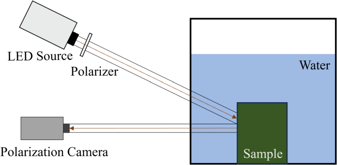
Experimental setup for underwater imaging.

The photographed sample is placed inside a transparent PMMA tank (40 × 40 × 40 cm), which is poured into clean water, followed by colored ink and milk to simulate the absorption and scattering effects. In this setting, we collect 240 sets of images consisting of polarimetric images captured in colored turbid water and corresponding intensity images captured in clean water, which are regarded as ground truths. We pour blue, green, and yellow ink to simulate multiple water types, and we pour milk of different amounts to simulate different levels of turbidity. Hence, the dataset consists of images from three domains, each of which is subdivided into four turbidity levels. In addition, a variety of objects such as plastic disk and color card, metal coin and ruler, and seashells are used to ensure diversity of content. We expand another 720 sets of images by rotating, and all images are resized to 160 × 160. Ultimately, this dataset, which simultaneously has different turbidity, water types, and colorful scenarios, is the richest dataset known to us and is large, with a total of 960 images and 320 of each water type. Examples of our acquired images are shown in Fig. 3, where domain 1 and domain 2 are trained by UPD-Net, thus called source domains, domain 3 is only for testing the generalizability of the trained model, thus called the unseen domain, and it is worth mentioning that, we also acquire polarization images in a real lake (viewed as domain 4). Total images of bluish and greenish domains are divided into training, validation, and testing sets by 2:1:1.

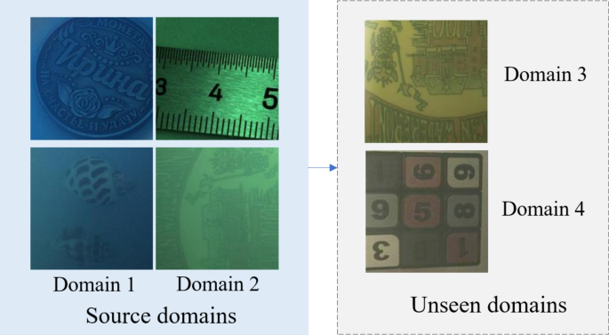
Examples of acquired images in four domains.

Network

Innovatively introducing domain-adversarial learning for the first time into underwater polarimetric imaging, we propose an underwater polarimetric color image recovery network for different environments, named UPD-Net, as shown in Fig. 4. It is a generative adversarial network consisting of multi-encoder (E), decoder 1 (D₁), decoder 2 (D₂), discriminator (J), and water-type classifier (C). Among them, E and D₁ form the generator (G), D₁ and D₂ have the same network structure. Multi-encoder and dual-decoder are designed by improving on U-Net⁴³, a commonly used network based on a single encoder-decoder that outputs images utilizing local and global information via skip connections. Because of the need for multi-polarization information fusion, we designed a Multi-encoder U-Net, where each encoder is responsible for generating a feature vector of one polarimetric image, and three vectors are connected to the latent vector by the concatenation concat. To be able to preserve not only the desired content but also the polarization information that needs to be mined and exploited during the encoding process, we include a parallel decoder D2 in addition to the decoder D1, which is used to output the DoLP image, which is a representation of the polarization information. This oversees that our network mines more polarization information from the raw polarimetric images.

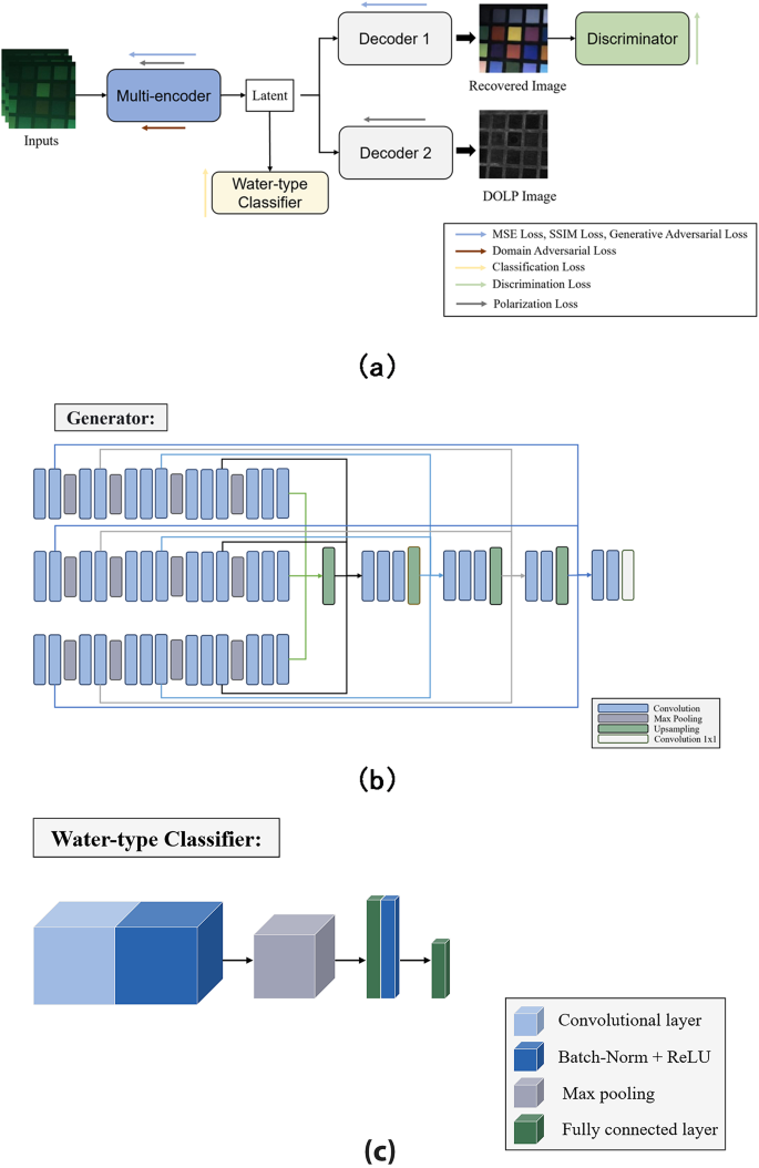
(a) The architecture of the UPD-Net; (b) the generator; (c) the water-type classifier.

Since the network aims not only at satisfactory image recovery but also to generalize to images of different water types, which are viewed as multiple domains, we introduce a novel application of a water-type classifier along with the generator and the discriminator. The water-type classifier is a neural network that aims to classify the water type of the given input images from the latent vector extracted from E. The distribution of images in different water types is different, and such diversity makes it hard to train a single model to recover images of various types, especially the ones unseen in training. Whereas the scene content unrelated to the water body is what the model needs to recover, thus the encoders are expected to produce domain-agnostic feature representations, specifically, the feature vectors are ideally only related to scene content and not to the water body. To achieve this goal, the water-type classifier is expected to become increasingly incapable of determining the water type of the input image based on the encoded feature representations during the training process. This process, known as domain-adversarial learning strategy, is similar to generative-adversarial learning strategy, the generator is expected to generate images that are increasingly not recognized by the discriminator as generated images but are mistaken for ground truths, whereas the E is similar to the generator and the C is similar to discriminator. Employing these two adversarial learning strategies, we use the learned domain-agnostic features to generate recovered underwater images closed to ground truths.

To optimize the water-type classifier, we adopt classification loss \({{\text{L}}_{\text{c}}}\):

where \({\text{I}}\) is distorted images, \({\text{Z}}={\text{E}}\left( {\text{I}} \right)\) and \({\text{T}}\) is the number of types, which is 2 in this work, \({\text{~}}{{\text{y}}_{\text{t}}}=1\) if \({\text{c}}={\text{C}}\) else \({{\text{y}}_{\text{t}}}=0\). \({{\text{L}}_{\text{c}}}\) is the cross entropy of the distribution of the water type \({\text{t}}\) predicted by \({\text{C}}\).

To optimize the generator, we adopt four losses: a Domain Adversarial Loss (\({{\text{L}}_{\text{d}}}\)), an MSE Loss (\({{\text{L}}_{\text{m}}}\)), an SSIM Loss (\({{\text{L}}_{\text{s}}}\)), and a Generative Adversarial Loss (\({{\text{L}}_{\text{g}}}\)).

Domain Adversarial Loss,

MSE Loss,

SSIM Loss,

Generative Adversarial Loss,

and Polarization Loss,

where\({\text{~}}{{\text{L}}_{\text{d}}}\) is the negative entropy of the distribution of the water type \(\left( {\text{t}} \right)\) predicted by \({\text{C}}\), and backpropagated only to update the E. \(\{ {\text{I}}_{{\text{i}}}^{{{\text{out}}}},{\text{~i}}=1,{\text{~}}2,{\text{~}} \ldots {\text{~*}},{\text{~N}}\}\) means the output recovered image and \(\left\{ {{\text{I}}_{{\text{i}}}^{{{\text{gt}}}},{\text{i}}=1,{\text{~}}2,{\text{~}} \ldots {\text{~*}},{\text{~N}}} \right\}\) the corresponding ground truth, \({{\text{L}}_{\text{m}}}\) and \({{\text{L}}_{\text{s}}}\) are calculated based on pixel-wise and structural differences, respectively. \(\{ {\text{I}}_{{\text{i}}}^{{{\text{raw}}}},{\text{~i~}}={\text{~}}1,{\text{~}}2,{\text{~}} \ldots {\text{~*}},{\text{~N}}\}\) denotes the input raw image, \({\text{G}}\) attempts to fake the discriminator and \({\text{J}}\) tries to recognize the generated images from the ground truths. Additionally, \(\{ {\text{DOLP}}_{{\text{i}}}^{{{\text{out}}}},{\text{~i}}=1,{\text{~}}2,{\text{~}} \ldots {\text{~*}},{\text{~N}}\}\) means the output DOLP image and \(\left\{ {{\text{DOLP}}_{{\text{i}}}^{{{\text{gt}}}},{\text{i}}=1,{\text{~}}2,{\text{~}} \ldots {\text{~*}},{\text{~N}}} \right\}\) the corresponding ground truth. \({{\text{L}}_{\text{m}}}\) and \({{\text{L}}_{\text{p}}}\) are calculated based on pixel-wise. We use the following summation of the above loss functions, as the Total-loss \({\text{L}}\), to backpropagate through the generator:

where \(\:{\upalpha\:}\), \(\:{\upbeta\:}\), \(\:{\upgamma\:}\), \(\:{\updelta\:}\), and ρ are the weights of \({{\text{L}}_{\text{d}}}\), \({{\text{L}}_{\text{m}}}\), \({{\text{L}}_{\text{s}}}\), \({{\text{L}}_{\text{g}}}\) and \({{\text{L}}_{\text{p}}}\), respectively, and the setting of the weights depends on the pre-training performance. Our network is implemented in the PyTorch framework, trained and tested by the NVIDIA GeForce RTX 4090 GPU. We utilize the Adam optimizer with a batch size of 4 to update the network parameters. The learning rate is initially set to 5e–5 and decays exponentially at a rate of 0.6. In the training process, we first train the generator to ensure that the feature vectors generated by the encoders are meaningful by utilizing \({{\text{L}}_{\text{m}}}\), \({{\text{L}}_{\text{s}}}\), \({{\text{L}}_{\text{g}}}\) and \({{\text{L}}_{\text{p}}}\). Then, we use classification loss to train the water-type classifier to reach a certain threshold of classification accuracy. Finally, the total loss \({\text{L}}\) is utilized to help the multi-encoder generate domain-agnostic feature representations to recover images in different domains. To avoid the common problems of mode collapse in generative adversarial networks and blurring of details in the generated images, we take measures to keep the network stable, such as doing batch normalization on the training data, lowering the weight of the Generative Adversarial Loss during the training process, and applying a low learning rate for the generator.