Machine learning-driven development of a stratified CES-D screening system: optimizing depression assessment through adaptive item selection | BMC Psychiatry

Recursive Feature Elimination (RFE) and linear regression model

Through Recursive Feature Elimination (RFE) combined with cumulative variance explanation (R²) analysis, this study identified 9 core items with significant predictive power from the CES-D-20 scale. Unlike traditional scale reduction methods that set a predetermined target for the number of retained items, our approach employs Recursive Feature Elimination (RFE), a data-driven method that systematically identifies the optimal item set. The selection of 9 items was based on detecting the inflection point in the R² curve, where additional items contributed minimal incremental variance explanation. This approach ensures that the retained items maximize predictive efficiency without relying on arbitrary cutoffs.

These items encompass multiple dimensions of depressive symptoms: emotional symptoms (C06 “I felt depressed”, C12 “I felt unhappy”, C18 “I felt sad”), cognitive symptoms (C09 “I thought my life had been a failure”), somatic symptoms (C02 “I did not feel like eating; my appetite was poor”, C07 “I felt that everything I did was an effort”), interpersonal symptoms (C14 “I felt lonely”, C19 “People were unfriendly”), and emotional vulnerability (C01 “I was bothered by things that usually don’t bother me”). Tese results can be found in Table 1.

The linear regression model constructed based on these 9 core items demonstrated excellent predictive performance. In tenfold cross-validation, the model achieved an average variance explanation (R²) of 0.9565, indicating that this abbreviated version effectively captures the severity of depressive symptoms reflected in the original scale. The model obtained an R² value of 0.9572 on the independent test set, further confirming its robust generalizability. As shown in Fig. 2, the cumulative variance explanation rate plateaus when the number of features exceeds 9, suggesting that additional items provide limited marginal information, thus supporting the feasibility of scale simplification.

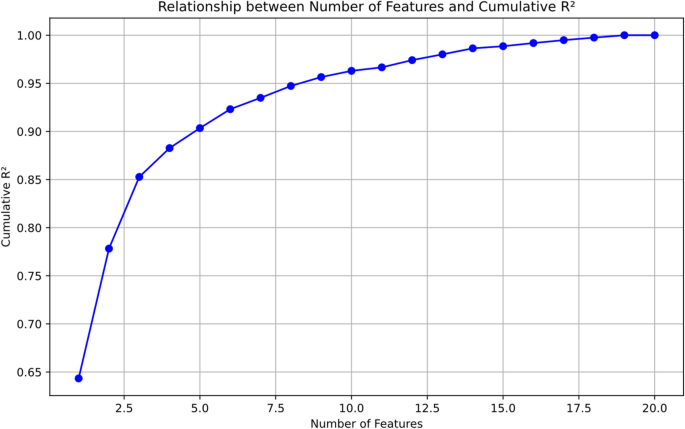
Relationship between number of features and cumulative variance explained (R.²): analysis of incremental predictive value with progressive feature addition. Model equation: Total = 0.6660 + 1.6584*C01 + 1.6832*C02 + 1.7542*C06 + 2.0579*C07 + 2.4517*C09 + 1.7700*C12 + 1.8957*C14 + 2.0316*C18 + 2.1980*C19

The final regression equation is as follows: Total = 0.6660 + 1.6584 × C01 + 1.6832 × C02 + 1.7542 × C06 + 2.0579 × C07 + 2.4517 × C09 + 1.7700 × C12 + 1.8957 × C14 + 2.0316 × C18 + 2.1980 × C19.

Analysis of the regression coefficients reveals that C09 (β = 2.4517) contributes most substantially to the prediction of total scores, followed by C19 (β = 2.1980) and C07 (β = 2.0579), suggesting that cognitive symptoms (negative life evaluation), impaired social functioning, and somatic symptoms may be critical indicators in assessing the severity of depression among adolescents.

Feature selection and classification model development

Through Recursive Feature Elimination analysis, we successfully identified a simplified yet efficient subset of CES-D items for predicting clinically significant depressive symptoms. The analysis revealed that among the original 20 items, only 4 core items were necessary to achieve excellent predictive performance. These four items are C18, C09, C06, and C19, encompassing key dimensions of emotional and cognitive depressive symptoms.

The logistic regression model constructed based on these four core items demonstrated outstanding diagnostic performance, achieving an Area Under the ROC Curve (AUC) of 0.98. Using the Youden index, the optimal classification threshold was determined to be 0.5808. At this cutoff point, the model exhibited exceptional diagnostic metrics across all parameters: sensitivity of 0.9449, indicating accurate identification of 94.49% of individuals with clinically significant depressive symptoms; specificity of 0.9262, suggesting correct screening of 92.62% of individuals without significant depressive symptoms. The model achieved an F1 score of 0.9361, reflecting an excellent balance between precision and recall, with an overall accuracy of 93.55%, highlighting its robust classification capabilities. Tese results can be found in Table 2. The AUC values and various diagnostic metrics under different feature combinations are shown in Figs. 3 and 4.

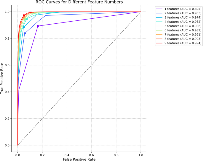
ROC curves analysis for different feature combinations: comparison of classification performance with incremental feature addition from core items

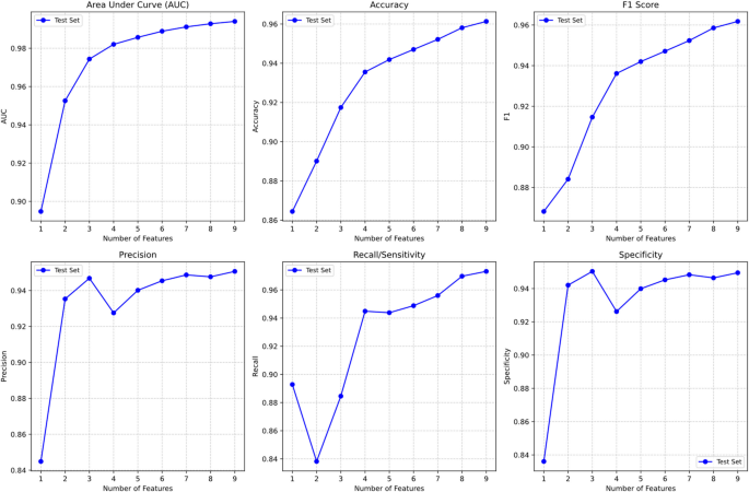
Multi-metric evaluation of model performance: changes in classification metrics (AUC, accuracy, F1 score, sensitivity, specificity, precision) with increasing item numbers

The final logistic regression prediction equation is:

Here, p represents the probability of an individual’s CESD total score being ≥ 16, while C18, C09, C06, and C19 represent the original scores (0–3 points) for their respective items. The regression coefficients indicate comparable predictive contributions from these items, underscoring their balanced importance in the assessment process.

Comparative analysis of multiple classification models

To determine the optimal classification algorithm, we conducted rigorous statistical comparisons among three machine learning models. One-way Analysis of Variance (ANOVA) revealed significant performance differences between models (F = 267.1417, p < 0.001). Subsequent Tukey HSD post-hoc tests demonstrated comparable performance levels between logistic regression and random forest models (p = 0.9996, 95% CI containing 0), while both significantly outperformed the support vector machine model (p < 0.001). These findings provided robust statistical evidence for model selection. For detailed comparison results, please refer to Fig. 5 and Table 3.

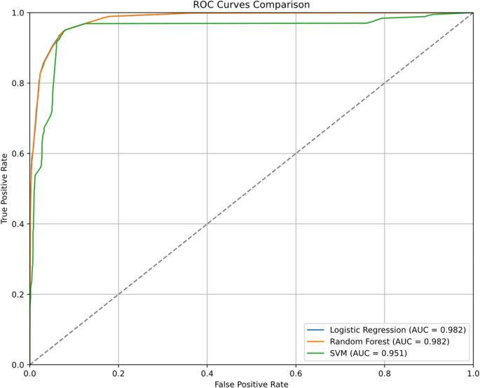
Comparative ROC curves analysis: performance comparison of logistic regression, random forest, and support vector machine models using four core items

Between the two models with comparable performance, logistic regression demonstrated distinct advantages. Primarily, as a linear model, it exhibits low computational complexity, particularly suitable for prediction tasks with fewer features. More importantly, logistic regression offers excellent interpretability, allowing for intuitive quantification of feature contributions to predictions through regression coefficients. This transparency holds particular significance in mental health screening applications, enabling clinicians to understand and interpret the sources of predictive outcomes.

In contrast, while the random forest model can capture non-linear relationships between features, its “black box” nature limits the intuitive interpretation of the model.

Based on this comprehensive analysis, we selected logistic regression as the final predictive model. This choice was driven not only by its superior predictive performance but, crucially, by its outstanding interpretability and practicality—characteristics that hold substantial value in developing a simplified yet effective screening tool for depressive symptoms.

External validation

Children and adolescents group validation

To assess the model’s generalization performance in child and adolescent populations, we conducted rigorous external validation using four independent samples. Specifically, we first identified nine most influential features through Recursive Feature Elimination (RFE) from the original dataset, then extracted these features from new datasets. During data preprocessing, we calculated total scores and eliminated instances with missing values to ensure data completeness. Subsequently, we applied the fitted linear regression model for prediction and comprehensively examined its generalization capability through multiple evaluation metrics. In terms of explanatory power, the model demonstrated excellent performance across all validation samples of children and adolescents. The R² reached 0.957 for CPHG single-parent family samples (n = 48,128), 0.962 for CPHG left-behind children T2 samples (n = 133,904), 0.937 for CLDS adolescent T1 samples (n = 1,075), and 0.947 for T2 samples (n = 742) (Table 4).

To validate the four-feature classification model, we extracted these features from new datasets and applied the fitted logistic regression model for classification. The results demonstrated excellent classification performance across all samples (Table 5, Fig. 6). The CPHG single-parent family sample showed outstanding performance with an accuracy of 0.918, sensitivity and specificity of 0.947 and 0.911 respectively, F1 score of 0.825, and an AUC of 0.979. Similarly, the CPHG left-behind children T2 sample exhibited remarkable results with an accuracy of 0.928, sensitivity and specificity of 0.955 and 0.921 respectively, F1 score of 0.838, and an AUC of 0.983. The CLDS database also yielded reliable validation results across two time points: T1 sample (n = 1,075) achieved an accuracy of 0.908, F1 score of 0.736, and AUC of 0.977; T2 sample (n = 742) showed an accuracy of 0.921, F1 score of 0.805, and AUC of 0.975. Notably, sensitivity remained above 0.95 across all samples, indicating stable depression risk identification capability. The consistently high accuracy rates above 0.90 across all samples further confirmed the model’s robust classification performance in child and adolescent populations.

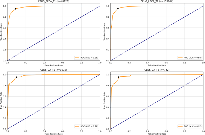
Cross-sample validation of four-item classification model: ROC curves analysis across different databases and time points

The model’s predictive probability calibration was evaluated through calibration curves (Fig. 7). The simplified scale demonstrated good calibration performance across multiple child and adolescent samples. Specifically, in the CPHG single-parent children (CPHG_SPCA_T1) sample, the calibration curve closely approximated the ideal 45-degree diagonal line, with a Brier score of 0.0579, indicating high consistency between predicted probabilities and actual observed outcomes. In the CPHG left-behind children follow-up sample (CPHG_LBCA_T2), the model also exhibited excellent calibration performance, with a Brier score of 0.0517 and high concordance between the calibration curve and diagonal line.

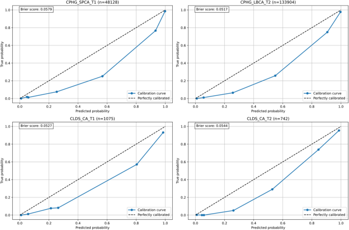
Calibration plot analysis: assessment of predicted probability accuracy across different samples and time points

Analysis of the CLDS adolescent samples further validated the model’s robustness. Despite the relatively small sample size (n = 1,075) at baseline measurement (CLDS_CA_T1), the calibration curve showed good fit with a Brier score of 0.0527. At the two-year follow-up measurement (CLDS_CA_T2), the model maintained stable calibration performance with a Brier score of 0.0544. Notably, across all samples, the calibration curves demonstrated optimal fitting in the medium to high-risk range, which precisely covers the most critical risk assessment interval in clinical decision-making.

The calibration curve analysis results indicate that the simplified scale, constructed from four core items, not only possesses good discriminative ability but also accurately estimates individual depression risk probabilities, which is crucial for risk assessment and intervention decisions in clinical practice. The low Brier scores (all < 0.06) further confirm the reliability of the model’s predictions, supporting the practical value of this simplified scale as a screening tool for adolescent depressive symptoms.

In the clinical application assessment for child and adolescent populations, decision curve analysis revealed significant screening value of the simplified CESD scale, as shown in Fig. 8. Specifically, in two large-scale populations—the CPHG single-parent children (n = 48,128) and left-behind children follow-up samples (n = 133,904)—the model demonstrated excellent and consistent net benefit performance. When risk thresholds ranged between 0.2 and 0.8, the model’s decision curves significantly outperformed both extreme strategies of “treat all” and “treat none,” providing superior options for clinical decision-making.

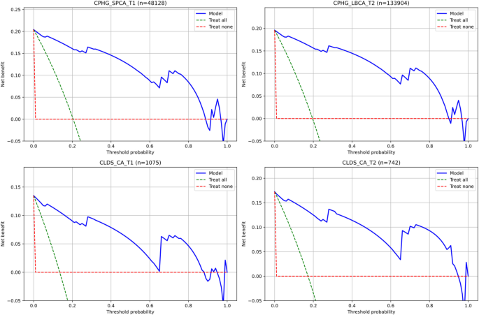
Decision curve analysis: net benefit assessment of the screening system across different risk thresholds in various population samples

Analysis of the CLDS adolescent samples further strengthened these findings. In both baseline (n = 1,075) and two-year follow-up (n = 742) data, despite relatively smaller sample sizes, the model maintained stable advantages in decision curves. Notably, the model showed maximum net benefit in the clinically critical decision interval of 0.3–0.6, a characteristic particularly significant for balancing screening sensitivity and specificity.

Particularly noteworthy is the model’s demonstration of robust decision curve characteristics across child and adolescent populations of varying sizes and backgrounds. This cross-sample consistency highlights its universality as a depression symptom screening tool. The stable trajectory of net benefit curves indicates that this simplified scale can provide reliable guidance for clinicians’ decisions across different risk thresholds, effectively enhancing early identification efficiency of depressive symptoms.

Cross-age group validation

To comprehensively assess the model’s applicability across different age groups, this study employed longitudinal data from various age cohorts within the CLDS database for validation. The validation sample encompassed three age groups: early adulthood (19–30 years), middle adulthood (31–65 years), and late adulthood (> 65 years). For each age group, data included baseline measurements from 2016 (T1) and follow-up measurements from 2018 (T2).

Regarding the linear regression models, the nine core features demonstrated exceptional explanatory power across all age groups in the validation samples. As shown in Table 6, the variance explained (R²) for the early adulthood group reached 0.951 and 0.950 in the baseline and follow-up samples, respectively. The middle adulthood group maintained stable R² values of 0.952 and 0.951, while the late adulthood group showed R² values of 0.952 and 0.947. These findings indicate that the simplified scale exhibits significant and consistent effectiveness in explaining depressive symptom variance across all age groups, with R² values consistently maintaining high levels above 0.94 across all samples.

As shown in Table 7 and Fig. 9, in validating the four-feature classification model, all age groups demonstrated excellent and stable predictive performance. The early adulthood sample (CLDS_A) performed exceptionally well in both baseline (n = 3,207) and follow-up (n = 2,052) measurements, achieving AUC values of 0.980 and 0.977, respectively, with accuracy maintained around 0.93, and both sensitivity and specificity remaining above 0.93. The middle adulthood sample (CLDS_B), which had the largest sample size (baseline n = 15,758; follow-up n = 12,697), also showed satisfactory validation results, with AUC values of 0.976 and 0.975 for baseline and follow-up measurements, accuracy maintained around 0.92, and both sensitivity and specificity exceeding 0.91. Although the late adulthood sample (CLDS_C) had a relatively smaller sample size (baseline n = 948; follow-up n = 955), the model performance remained robust, with AUC values of 0.983 and 0.975 for baseline and follow-up, achieving accuracy rates of 0.953 and 0.915, respectively.

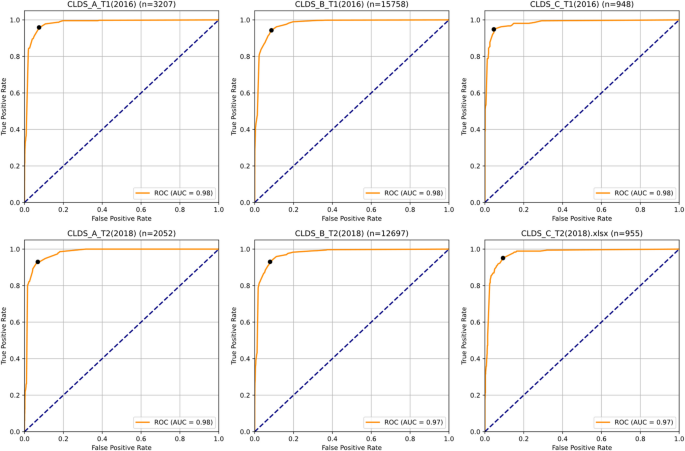
Age-stratified ROC curves analysis: classification performance of four-item model across different age groups and time points

Cross-age group comparative analysis revealed that both linear regression and classification models maintained high predictive accuracy across all age groups. Linear regression results showed minimal variation in R² values across age groups (range: 0.947–0.952), indicating model stability in explaining depressive symptoms across age spans. Regarding classification performance, accuracy rates were maintained between 0.915–0.953 across all samples, demonstrating excellent risk identification capability (sensitivity 0.930–0.959). Notably, the late adulthood sample showed the most outstanding overall performance in the 2016 baseline measurement, achieving a precision of 0.855 and an F1 score of 0.899, suggesting particularly ideal predictive capability in the elderly population. While the middle adulthood sample had the largest sample size, its stable performance across all indicators demonstrated the model’s reliability in large-sample settings. The early adulthood sample maintained high predictive performance at both time points, with the follow-up sample showing an improved F1 score (0.830) compared to baseline (0.796), indicating stable or even enhanced predictive capability over time.

The model’s predictive accuracy across different age groups and time points was evaluated through calibration curves and Brier scores (Fig. 10). Results demonstrated good and stable calibration performance across all six validation datasets. Brier scores ranged from 0.0398 to 0.0557, indicating excellent predictive accuracy (all scores < 0.10). Specifically, in the 2016 datasets, CLDS_C_T1 (n = 948) exhibited the best calibration performance with a Brier score of 0.0398, followed by CLDS_A_T1 (n = 3,207) with 0.0504 and CLDS_B_T1 (n = 15,758) with 0.0557. The 2018 datasets showed similar patterns, with Brier scores of 0.0502 for CLDS_A_T2 (n = 2,052), 0.0553 for CLDS_B_T2 (n = 12,697), and 0.0528 for CLDS_C_T2 (n = 955).

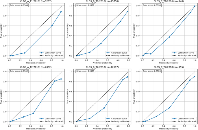
Age-stratified calibration analysis: assessment of predicted probability accuracy across different age groups and time points

The calibration analyses specifically addressed concerns about potential score inflation across different response patterns. The close alignment between predicted probabilities and observed outcomes (Brier scores ranging from 0.0398 to 0.0579) indicates that the simplified versions maintain accuracy regardless of whether participants scored highly on the selected items or showed different response patterns. This robustness is further supported by the consistent performance across diverse validation samples, suggesting that the models effectively capture depression severity without systematic bias toward particular response patterns.

Calibration curves consistently demonstrated a slight tendency toward risk overestimation, particularly in the low probability range (0–0.4), while showing better calibration performance in the high probability range (0.8–1.0). This systematic pattern remained consistent across different age groups and time points, indicating stable model performance. The findings suggest that the model performs exceptionally well in identifying high-risk individuals, although it slightly tends to overestimate actual risk in low-risk populations.

Decision Curve Analysis (DCA) was conducted on six independent validation datasets to further evaluate the clinical utility of the simplified CESD scale (Fig. 11). Results demonstrated significant clinical net benefit of the four-feature logistic regression model across all validation samples. Specifically, in the 2016 baseline data, the decision curves for early adulthood (CLDS_A_T1), middle adulthood (CLDS_B_T1), and late adulthood (CLDS_C_T1) samples outperformed both extreme strategies of “treat all” and “treat none” across most threshold probabilities (approximately 0.2–0.8). The model maintained stable and substantial net benefits within the critical decision threshold range of 0.2–0.8. The 2018 follow-up data validation results (CLDS_A_T2; CLDS_B_T2; CLDS_C_T2) exhibited similar patterns, indicating good temporal stability in the model’s clinical value.

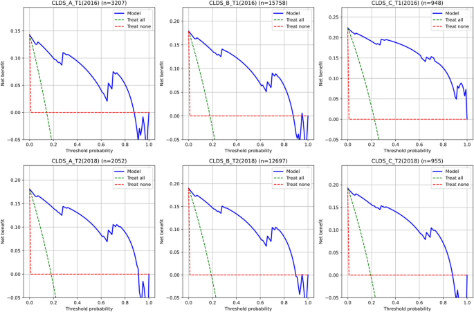
Age-stratified decision curve analysis: net benefit assessment across different risk thresholds for various age groups

Notably, the model demonstrated maximum net benefit within the threshold probability range of 0.3–0.6, which precisely corresponds to the most commonly used decision threshold range in clinical practice. This finding corroborates the previous calibration curve analysis results, further supporting the simplified scale’s advantages in identifying moderate to high-risk individuals. Cross-age group comparisons revealed comparable decision benefits across all age groups despite substantial differences in sample sizes, highlighting the model’s broad applicability. These results align with the model’s excellent performance in discrimination (AUC) and calibration (Brier scores), collectively confirming the practical value of the simplified CESD scale as a depression symptom screening tool.