
Intelligent agricultural robotic detection system for greenhouse tomato leaf diseases using soft computing techniques and deep learning

This section comprises three subsections, each of which explains the different components involved in developing an agricultural robot for tomato plants.
Trajectory design based on fuzzy controller for an agricultural robot
The agricultural robot was designed to travel easily between tomato rows, as shown in Fig. 1. The tomato plant’s maximum height is about 1.2 m, and the distance between rows is 60 cm, while the distance between tomato plants is 40 cm. The robot includes a basement with a dimension of 40 × 40 cm, MPU 6050, and ultra-sonic sensor SRF04 to avoid low-position obstacles. Additionally, a camera was used for navigation and learning purposes. A 2D camera was used to take pictures of the tomato leaf, while the Intel RealSense depth camera D435 was used to implement the simultaneous localization and mapping (SLAM) task. The proposed navigation was implemented in the Ubuntu 16.04 LTS operating system running on the Robot Operating System (ROS) Kinetic.

Robot design (left) and real robot (right).

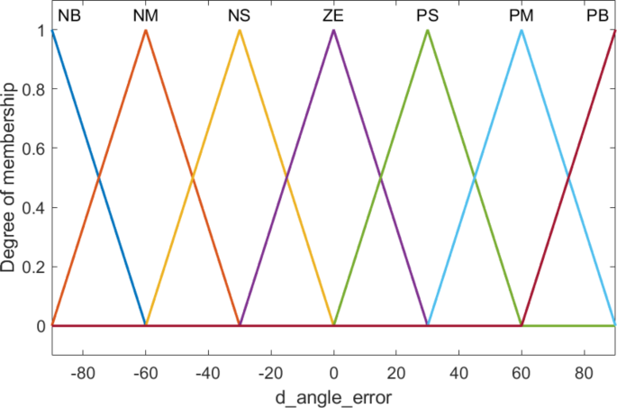
The angle error triangular membership functions.
For the navigation task, the robot starts at the first corner of the greenhouse and fully travels through all tomato rows to take pictures and monitor the tomato plant. Fuzzy control is used, with the inputs being the angle error and the derivative of angle error. The angle error (angle_error) and the derivative of angle error is designed with physical values from − 900 to 900, including seven linguistic values corresponding to seven membership functions: NB (Negative Big), NM (Negative Medium), NS (Negative Small), ZE (Zero), PS (Positve Small), PM (Positve Medium), PB (Positve Big) as shown in Figs. 2 and 3, respectively.
The angle error derivative triangular membership functions.

The angular velocity triangular membership functions.
Corresponding to the two input variables angle error (angle_error) and angle error derivative (d_angle_error) is the output variable angular velocity with a physical value range from − 1.2 rad/s to 1.2 rad/s, including 7 linguistic values corresponding to 7 membership functions: NB (Negative Big), NM (Negative Medium), NS (Negative Small), ZE (Zero), PS (Positive Small), PM (Positive Medium), PB (Positive Big) as shown in Fig. 4. The fuzzy associative memory (FAM) table is presented in Table 1, while the fuzzy curve is shown in Fig. 5.

The fuzzy curve of the composite of angular velocity rules based on the two input variables.
Dataset and improved DCGAN
For this study, we utilized the PlantVillage dataset44, which consists of ten groups with healthy leaves and nine different leaf diseases (Bacterial spot, Early blight, Late blight, Leaf Mold, Septoria leaf spot, Two spotted spider mite, Target Spot, YellowLeaf Curl Virus, Tomato mosaic virus). Each image in the dataset has a resolution of 256 × 256 pixels, RGB color space, and is in JPG format. The original dataset was divided into two sets, a training set, and a validation set, in an 80:20 ratio for each class. Figure 6 shows examples of the ten classes in the original dataset.
GANs were first introduced in 201445, which consist of two models: a generator G and a discriminator D. The generator generates images for training purposes, while the discriminator distinguishes between real training images and generated images, as shown in Fig. 7. In this study, we proposed DCGAN for data augmentation. Figure 8 illustrates the structure of the two models, generator and discriminator, in the proposed improved DCGAN. The details of Generator and Discriminator are presented as follows:
Generator structure.
Input layer
Receives a random noise vector.
Dense layer
Converts this noise vector into a 3D tensor of larger size (16 × 16 × 512). This creates a small “image” but with many feature maps.
Reshape layer
Converts the tensor from vector form to spatial form to be processed by convolutional layers.
Conv2DTranspose layers
These layers perform “upsampling” (enlarging) of the image, gradually increasing the spatial dimensions (from 16 × 16 to 128 × 128). Conv2DTranspose is used with different filter sizes to progressively create a higher resolution image.
Residual blocks with concatenation: Includes two residual blocks, each performing a series of steps: Conv2D -> BatchNormalization -> LeakyReLU -> Conv2D -> BatchNormalization. The output of the block is then concatenated with the original input to retain the original information. These blocks help the model learn deeper features and retain information from previous layers.
Concatenate & upsampling
After the Residual Blocks, features from these blocks are combined and the size is further increased.
Output layer
The final layer is Conv2DTranspose with a tanh activation function, producing an RGB image of size 128 × 128 × 3. The tanh function normalizes the output values to the range [-1, 1], suitable for the Discriminator’s input format.
Discriminator structure:
Input layer
Receives an image of size 128 × 128 × 3 (RGB).
Conv2D layers
Used to progressively reduce the image size while extracting important features.
Spectral normalization
Applied to the Conv2D layers to normalize the spectral norm of the weight matrix, helping stabilize the training process and avoid gradient issues.
LeakyReLU
Used after each Conv2D layer to introduce non-linearity into the model, helping the model learn more complex features. LeakyReLU is chosen over ReLU to avoid the dead neuron problem.
Dropout layers
Used after convolutional layers to minimize overfitting by randomly dropping some connections in the network.
Flatten layer
After the Conv2D layers, the image is flattened into a vector before being fed into the final layer.
Output layer
The final layer is a single Dense layer, with the output being a scalar value representing the model’s confidence that the input image is real or fake.
The proposed improved DCGAN network includes several enhancement techniques:
Using Residual Blocks in the Generator helps preserve information through the deep layers of the network, improving the ability to generate detailed and complex features. In addition, spectral Normalization in the Discriminator is used to stabilize the Discriminator’s training process by normalizing weights in Conv2D layers, aiding the model in avoiding gradient issues and improving convergence. Moreover, Mixed Precision Training utilizes both 16-bit and 32-bit floating-point numbers during training to accelerate computation and reduce memory usage while maintaining model accuracy.
After DCGAN is trained on the original dataset, it is used to generate 500 images for each class. The generated images have the same resolution as the original image, PNG format, and RGB color space. Examples of synthetic images are shown in Fig. 9. Each class added 500 images after generating data using DCGAN, resulting in a total of 21,012 images (16204 for training and 4808 for validation). The classes of the augmented dataset and class-wise image distribution are represented in Table 2.

Examples of original dataset.


Improved DCGAN processing.

Examples of synthetic images.
Model training
We investigated four different transfer learning models, namely VGG-19, Inception-v3, DenseNet-201, and ResNet-152, on the original dataset, and selected the best model to train on the dataset enriched with improved DCGAN. After training the models on the initial dataset, we obtained the training curves and the accuracy of the models. The training curves of the models are shown in Figs. 10, 11, 12 and 13. The values of validation accuracy for these models are 92.32%, 90.83%, 96.61%, and 97.07% respectively with the original dataset for nine tomato leaf disease classes. As a result, we chose ResNet-152 to build a disease leaves classification model with data enriched by improved DCGAN.

VGG19 classification models results.

Inception-V3 classification models results.

DenseNet 201 classification models results.

ResNet-152 classification model results.
link


