Incorporating soil information with machine learning for crop recommendation to improve agricultural output

Despite recent attempts to find solutions, challenges still exist in providing effective crop recommendations. The proposed solution aims to address these challenges by developing machine learning models that consider vital parameters like N, K, P, rainfall, temperature, humidity, and pH, directly impacting farming. The objective is to suggest a broader range of suitable crops for the season, reducing farmers’ difficulties in crop selection and ultimately increasing yield. The proposed model recommended the best crops for soil. The integration of agriculture and machine learning promises to advance the agriculture field by enhancing optimizing and yield resource utilization. The dataset undergoes comprehensive preprocessing, using a training split ratio is 80% and a testing ratio is 20%. The workflow of the proposed methodology is given in Figure 1. The methodology comprises several phases including collection of data, preprocessing, explorative data analytics, correlation, splitting of dataset, employing machine learning models, and crop recommendation.
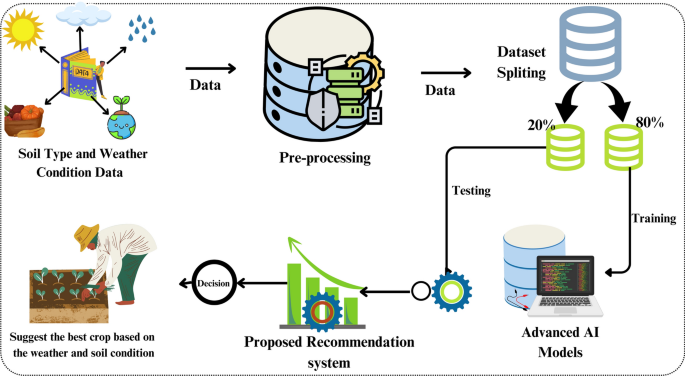
The methodological infrastructure of our proposed research suggests the best crop.
Phase 1: Dataset collection
Utilizing data from previous years plays a vital role in forecasting current performance. We collect historical data13,14 from reliable sources like Kaggle and IEEE Dataport. The dataset was originally collected by the Agricultural research stations and weather stations from Islamabad Capital of Pakistan. The dataset incorporates information on N, K, and P levels in the soil, alongside temperature and rainfall measurements, elucidating their impact on crop growth. This dataset serves as a valuable resource for formulating data-driven recommendations to optimize nutrient and environmental conditions, ultimately enhancing crop yield. The dataset contains 2200 instances. It includes twenty-two different crops: maize, rice, chickpeas, pigeon peas, broad beans, kidney beans, mung beans, lentils, pomegranates, black beans, bananas, grapes, watermelon, mangoes, melon, oranges, cotton, papaya, apples, coffee coconut, and jute.
Phase 2: Data preprocessing
By using categorical values such as labels in the datasets are managed using the label encoding method. The analysis of descriptive features related to the dataset is presented in Table 2. It provides details on attributes, attribute types, and their corresponding descriptions15,16.
The dataset has seven features while the 8th attribute is the label of the class which indicates the crop name. Each attribute shows different features of the dataset which helps to recommend a specific crop. The ’N’ indicates Nitrogen content, ’P’ shows the quantity of Phosphorus, and ’K’ refers to the Potassium content. ’Temperature’ shows soil temperature in Fahrenheit, ’Humidity’ is the amount of water content, ’pH’ shows soil’s acidic or alkaline level and varies between 5.5 to 6.5 while the ’Rainfall’ feature shows the quantity of rain in mm.
Phase 3: Exploratory data analytics
Exploratory data analytics refers to the process of data analytics, using data sets, graphical representation, and content analytics. Feature relationship analytics and data visualization methods contribute to the suggestion process of the proposed models. In Table 3 are shown the results of the data analytics process. Special statistics calculated mean, standard deviation (std. varies), minimum, 25%, 50%, 75%, and maximum. Inspection shows that the file contains 2200 lines of data. This analysis provides insights related to the central tendency of data, its distribution, variability, and outliers.
Table 3 provides quantitative information about the dataset concerning standard deviation, minimum values, maximum values, etc. Often, such information is useful and can be used to improve the performance of models. The mean value indicates the average value of data for each feature while min., and max. values indicate the minimum and maximum values for the data given for each feature. Similarly, standard deviation is taken from all the data for each feature, and 25%, 50%, and 75% show the first, second, and third quartiles for each feature.
Figure 2 provides a visual comparison of different parameters (nitrogen, phosphorus, potassium). It helps understand the relationship between these parameters and the proposed crop, making it easier to make decisions such as crop selection and management in agriculture.
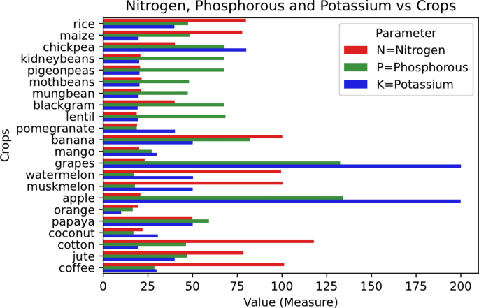
Distribution of N, p, and K input analysis with respect to various crops.
In Figure 3 the bar chart visually shows the relationship between three parameters (temperature, humidity, and pH) and their impact on crop recommendations. Each bar on the chart shows the average of one of these parameters.
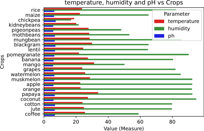
Variation in temperature, humidity, and pH input analysis with respect to various crops.
In Figure 4the bar chart shows the relationship between one parameter rainfall and their impact on crop recommendations. Each bar on the chart shows the average of one rainfall. Exploratory analysis exhibits that soil pH, nitrogen, phosphorus, potassium, temperature, and rainfall contents are very important for farmers to determine, which kind of crops can be fully grown in soil type17.
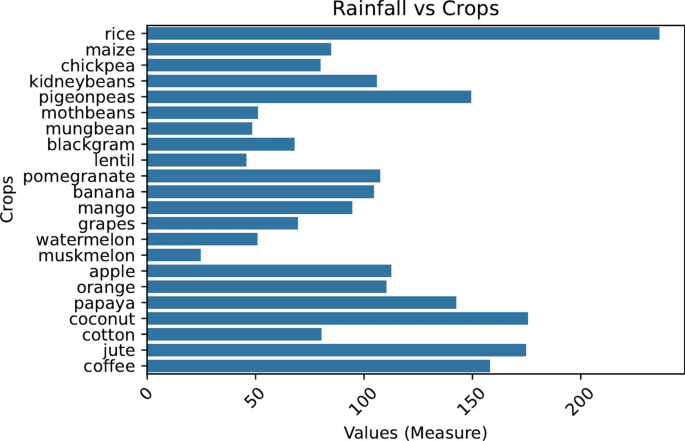
The rainfall distribution and various crops.
Phase 4: Correlation analysis
While designing machine learning models, it is important to select appropriate features for training models that are strongly related to the target variable. The chosen features correlation analysis is illustrated in Figure 5, indicating that all selected features exhibit a positive correlation with each other. Notably, the K and P features exhibit a high correlation of 0.74. This analysis signifies that the features within our research dataset exhibit favorable correlation values, making them well-suited for training machine learning models, particularly for crop recommendation.
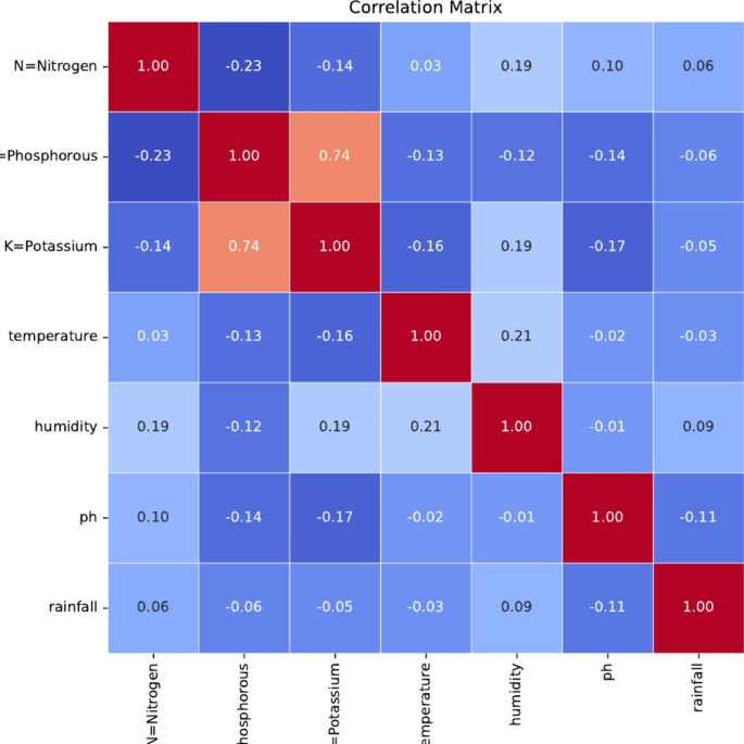
Evaluation of the relationship between input features within a dataset bee-line correlation analysis.
The classification analytics of the bar plot is illustrated in Figure 5. The analytics of different features of the collected data. It shows that each feature has a different impact on the crop, demonstrating the importance of features in predicting each bar line.
Phase 5: Dataset splitting
To remove the overfitting of the model and assess the trained models on seen test data, data splitting is employed. The data is divided into 2 segments for testing and training using the train-test-split function of the sklearn library in Python, with an 80:20 ratio. The model is trained using the larger 80% portion, while a 20% portion of the dataset (2200 instances) is used for testing machine learning models’ performance.
Phase 6: Utilized machine learning techniques
This section examines the machine-learning models18,19,20 employed for best crop recommendations based on temperature and rainfall. The working mechanism of machine learning models is described, with a focus on six recommended machine learning models in our research study.
Extra trees classifier
Similar to random forests, additive tree classifiers are a popular ensemble learning method used in agricultural systems to recommend crops based on soil type and precipitation21. This classifier builds multiple decision trees using a random subset of the training data and a random subset of the features. An additional tree classifier for crop recommendation can be expressed as:
$$\begin{aligned} Z(x) = \ frac{1}{T} \sum _{t=1}^{T} z_t(x) \end{aligned}$$
(1)
where Z(x) represents the expected cleanup recommendation for input rows x. Each \(z_t(x)\) is a decision tree trained on a random subset of the training dataset and features. The final prediction is obtained by aggregating the predictions of all decision trees, often through majority voting.
Multilayer perceptron
The MLP is a type of artificial neural network commonly used in agricultural systems for crop recommendation based on features such as soil type and rainfall22. Here’s the formulation of an MLP for crop recommendation.
Let X represent the input feature matrix, where every row corresponds to a plot of soil, and each column represents a specific feature such as soil type, rainfall, temperature, etc. Each row is denoted as \(x_i \in \mathbb {R}^d\), where d is the number of features.
Let Y be the corresponding target class variable, indicating the recommended crop for each plot of land. Each target class variable is denoted as \(y_i \in {0, 1, \ldots , C}\), where C is the number of crop classes.
Decision tree
The DT model has emerged as a forceful tool in agricultural systems for crop recommendation based on soil type and rainfall. By leveraging a tree-like structure, the DT model effectively captures the relationships and patterns inherent in environmental features, facilitating accurate recommendations for crop selection. Through recursive partitioning, the model partitions the dataset into inferior subsets based on specific features, ultimately generating decision rules that enable the classification of plots of land as suitable for cultivating certain crops23.
Consider a dataset \(\mathscr {S}\) comprising M instances representing plots of soil, each characterized by a rest of features \(\textbf{X}_j\), and labeled suitable (\(Y_j = 0\)) or unsuitable (\(Y_j = 1\)) for a particular crop. The objective is to build a DT model to classify landing instances of soil plots. At each decision tree node, the optimal splitting criterion needs to be determined. Gini impurity is one commonly used measure, denoted as
$$\begin{aligned} \text {Gini}(\mathscr {G}) = 1 – \sum _{b=0}^{C-1} \left( \frac{|\mathscr {G}_b|}{|\mathscr {G}|}\right) ^2 \end{aligned}$$
(2)
where, C shows the number of classes, \(\mathscr {G}_b\) denotes the subset of rows inclusion to class b, and \(|\mathscr {G}|\) indicates the total number of rows in \(\mathscr {G}\).
Logistic regression
LR24,25 models are widely used in agricultural systems to recommend crops based on environmental factors like rainfall and soil type. LR models excel at binary classification tasks, accurately recommending crops that are suitable or unsuitable for cultivation based on input data.
In the context of crop recommendations, let us denote by X the characteristics of a particular piece of land, including soil type, precipitation, temperature, and other environmental variables. The binary variable Y indicates whether a particular crop is recommended to be grown in a particular region.
The LR model imagines an unbending relationship between traits and the likelihood of recommending a particular crop.
$$\begin{aligned} \log \left( \frac{L(y = 1 \mid x)}{1 – L(y = 1 \mid x)}\right) \end{aligned}$$
(3)
Random forest
The RF algorithm has obtained significant interest and adulation in agricultural systems for crop recommendations based on soil type and precipitation26,27..The ensemble learning method has shown optimistic accuracy in efficiently processing complex agricultural data. Combining the DT model RF effectively captures the patterns, relationships, and correlations in environmental characteristics to accurately recommend crops suitable for cultivation. X shows the feature matrix as input. Here, every row consists of a piece of land and every column shows a specific characteristic such as soil type, precipitation, temperature, etc. Every instance is indicated by \(X_j \in \mathbb {R}^f\). Where f is the number of objects. The corresponding target variable is shown with Y to the recommended crop for each land. Every target variable is indicated by \(Y_j \in \{0; 1;\ ldots; B\}\). In which B is the number of crop information.
RF models comprise a decision tree T, denoted \(r_t(x)\). Here \(t = 1; 2; \ ldots; A\). Every decision tree is trained to use a randomly selected subset of the agricultural dataset. The RF model integrates the prediction from all using the decision trees to predict the recommended crop for a new piece of land, denoted x. A majority vote obtains the final recommendation, and the recommended crop in which the mentioned target class collective mostly votes beyond all decision trees. RF model for crop recommendation is indicated as follows.
$$\begin{aligned} K(x) = \ frac{1}{R} \sum _{j=1}^{R} h_j(x) \end{aligned}$$
(4)
where K(x) shows the expected cleanup recommendation for input instance x.
Extreme gradient boosting classifier
XGBoost classifier is an algorithm of machine learning widely used in agricultural systems for crop recommendation placed on soil type and weather. Renowned for its efficiency, speed, and accuracy, XGBoost belongs to the boosting algorithm family28. The XGBoost algorithm iteratively constructs decision trees, with each subsequent tree aiming to rectify the errors of its predecessors. It amalgamates the prediction of numerous weary learners (individual DT) to produce the final recommendation.
The formulation for the crop recommendation problem using XGBoost can be expressed as follows:
$$\begin{aligned} \text {Target} = \sum _{j=1}^{m} \text {Loss}(\hat{Y}_j, Y_j) + \lambda \sum _{p=1}^{P} \Omega (f_p) \end{aligned}$$
(5)
where:
-
\(\text {Loss}(\hat{Y}_j, Y_j)\) signifies the inconsistency between the predicted values (\(\hat{Y}_j\)) and the actual values (\(Y_j\)) and measures the prediction error.
-
\(\Omega (f_p)\) represents the complexity penalty term applied to each decision tree (\(f_p\)), penalizing the model’s complexity.
-
P indicated the total number of trees in the novel ensemble.
-
\(\lambda\) serves as a regularization parameter, governing the trade-off between minimizing the prediction error and controlling the model’s complexity.
Phase 7: Fine-Tuning hyperparameters for models
To promote the performance of machine learning models, a systematic hyperparameter tuning process is implemented. To ensure the best recommendations, we use the iterative method a k-fold cross-validation process, to determine the optimal hyperparameters which divides the data into training, validation, and testing. Table 4lists the hyperparameters selected for the proposed method. The results of the analysis show that the negative agreement we identified was successful in accepting crops and achieved good performance29.
The primary reason for choosing systematic hyperparameter tuning for the proposed model was due to its complex architecture, which made it challenging to apply automated tuning methods effectively. We selected a manual, systematic approach to carefully explore and control the hyperparameters, such as learning rate, batch size, and number of hidden layers, before training the model.
The systematic tuning was guided by domain knowledge and iterative testing, allowing us to make informed decisions with relatively lower computational overhead. This approach helped us manage computational resources effectively by avoiding exhaustive searches or high-dimensional parameter spaces. Additionally, while there are many sophisticated hyperparameter tuning methods, such as grid search, random search, or Bayesian optimization, they can be computationally expensive. Since our primary goal was to establish a baseline performance, systematic tuning was a practical first step.
Phase 8: Proposed ensemble model
To improve decision-making by learning features, an ensemble model RFXG was implemented, combining more than one architecture, Like an RF and XGB model, and making an RFXG ensemble model. The experiments showed that RF and XGB performed well when we trained RF and XGB individually, so we combined RF and XGB to yield better results.
Combinations of RF and XGB were employed to model soil and weather parameters from the dataset using the hard-voting technique. We describe the operational rules of the implemented machine learning techniques ETC, MLP, DT, RF, XGB, and LR and introduce the ensemble model RFXG. Rather than encompassing all machine learning models, we strategically choose six benchmark models to represent various categories. These models encompass ETC for randomized decision trees, RF for ensemble learning, LR for binary classification, XGB for boosting ensemble, MLP for neural network-based learning, and DT for hierarchical classification. This selection aims to provide a comprehensive analysis, training each algorithm individually with the soil type data and evaluating their accuracy for comparison with the proposed ensemble learning model RFXG.
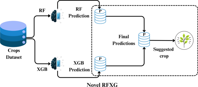
Ensemble machine learning model RFXG.
The RFXG model is proposed to improve prediction accuracy by accounting for data differences during model training. It combines RF and XGB algorithms using the advantages of simplicity, low data quality, and fast implementation. Unlike traditional methods, RFXG dynamically evaluates the importance of new data based on their similarity to the training context, without the need for an index. By integrating new machine learning technology in Figure 6. It combines the expression function of two algorithms to provide a unique hyperplane fusion. This method is capable of solving the overfitting problem and optimizing the dataset. RFXG’s architecture facilitates direct application to new data based on machine learning training and testing procedures. Although the principle remains the same, tuning the hyperparameters that make up the algorithm can improve the performance of different data sets.
The ensemble model combines RF and XGB based on the following points:
-
When analyzing the existing literature, tree-based models like RF and XGB are found to produce good performance for crop recommendations and similar tasks.
-
Their ensemble makes sense because RF’s ability to handle high-dimensional data and feature interactions when combined with XGB’s efficiency in handling large datasets and its robustness to outliers can provide better results than using an ensemble of other models.
-
Preliminary experiments showed that RF and XGB performed well as stand-alone models leading to joining them for better accuracy.
-
When combined, RF and XGB have improved feature representation due to RF’s feature importance and XGB’s feature interaction.
-
RF’s ensemble approach and XGB’s regularization can provide enhanced robustness.
-
Better handling of non-linear relationships is possible using RF’s decision trees and XGB’s gradient-boosting approach.
The dataset consisted of twenty-two different crops, turning it into a multi-classification task. Crop suitability, in this context. These conditions encompass various factors such as soil properties, climate, temperature, precipitation, and sunlight11. Recommending the best suitable crop using soil factors and environmental conditions empowers farmers to select the most suitable increasing productivity and improving resource utilization.
link


