Hyperspectral discrimination of vegetable crops grown under organic and conventional cultivation practices: a machine learning approach

Spectral reflectance measurements
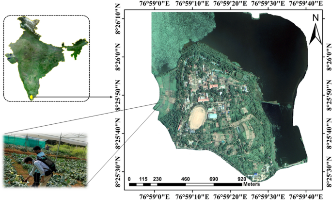
Kerala Agricultural University, India, established a center of excellence in organic farming to encourage and transform the regional landscapes from the prevailing conventional agricultural practices into organic ones. As part of the activities of promoting and producing quality organic crop inputs such as seeds, seedlings, organic fertilizers, pest and disease control agents, etc., numerous crops are routinely grown on the research farms of the College of Agriculture (CoA), Kerala Agricultural University, Thiruvananthapuram, India. The CoA has one of the largest certified organic research farming facilities in India, with crop-growing activities undertaken in multiple seasons throughout the year. For reference studies on the spectral distinctness of organic crops, we considered reflectance data acquisition on two types of crop growth experiments – (i) two crops, brinjal (Solanum melongena) and red spinach (Amaranthus dubius), grown under both the organic and conventional cultivation practices and (ii) crops grown under conventional cultivation practices. Seventeen different crops – vegetables, fruits, cereals, and spices belonging to nine different families of plants formed the crops sampled for measuring spectral reflectance. The list of crops and the cultivars used are detailed in Table 1. Except for banana (Musa acuminata) and chilli (Capsicum annuum), the crops were sown or transplanted in the winter season from 20 – 30 September 2022. Bananas and chili were planted in June and August 2022, respectively. The crops were cultivated based on the recommendations documented in the adhoc package of practices recommendations for organic farming18 and the package of practices recommendations: crops 201619. The agronomic practices related to providing nutrients and managing crop growth, such as pests, diseases, weeds, and contamination, were undertaken as prescribed in the aforementioned references. With a mean sea level of 15 meters, Thiruvananthapuram is a tropical climate region with an annual mean temperature of 25.7 °C. Predominantly from southwest monsoons, this region receives annual rainfall of about 2100 mm. Due to its favorable climatic and weather conditions, the region is suitable for growing various crops and up to three cropping seasons a year. The location map of the study site is shown in Fig. 1.
The spectral signatures were collected using two sets of hyperspectral spectroradiometer ((i) make: ASD, USA, Model: FieldSpec3; (ii) make: SVC, USA, model: HR1024i) to acquire the measurements under stable illumination conditions and with minimal temporal deviations. The ASD FieldSpec3 has a Full-Width-Half-Maximum (FWHM) of 3 nm at 700 nm, 10 nm at 1400 nm, and 10 nm at 2100 nm. The SVC HR1024i has 3.3 nm, 9.5 nm, and 6.5 nm, respectively. Both the instruments have a wavelength range that extends from 350 nm to 2500 nm and a field of view (FOV) of 25°. As per the phenological stage observed for different groups of the crops considered, spectral reflectance measurements were undertaken during 15–21 November 2022. The measurements were acquired on sunny days with clear skies between 11 and 1 pm. To ensure quality spectral measurement and minimize the influence of background reflectance, spectral measurements were recorded holding the optical tip of the sensor over the plant at a height varying between 5 and 25 cm depending upon the crop type and growth condition of the plant being sampled.

Location map of the study site used for acquiring in situ hyperspectral reflectance measurements (imagery: NRSC Bhuvan, Google Earth).
Multiple spectral reflectance samples were acquired for each crop based on the plant condition, intra-crop phenological variation, and spatial distribution. As an approximation of the measurement of solar irradiance required for calibration of the reflectance measurements, we acquired spectral measurements over a reference panel made of Barium Sulfate (BaSO4) at each measurement location and also adjusted according to the perceived changes in the illumination conditions. Filtered for outliers and extremities in the spectral variations, we obtained 536 spectral reflectance measurements for all the crops for further processing and analysis. The number of spectral reflectance measurements considered for each crop is listed in Table 2.
Pre-processing of spectra
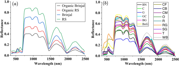
The raw spectral measurements were converted from radiance to reflectance by normalization against the white reference panel. As the raw spectra were distorted and contained small spikes, the Savitzky-Golay smoothening algorithm was applied to smooth the spectra. To establish baseline spectral data processing, we performed spectrum normalization and wavelength resampling to a uniform spectral interval of 5 nm, as the spectral measurements were obtained using two distinct instruments. After accounting for removing spectral outliers and measurement extremities, we retained reflectance measurements in 369 spectral channels spread across the optical range of the electromagnetic spectrum. Fig. 2 shows the mean reflectance spectra of crops considered for the study.

Mean reflectance spectra of considered crops: (a) organic vs. conventionally cultivated crops, and (b) other considered crops; RS (Red spinach), BN (Banana), C (Cabbage), G (Ginger), GC (Green Chilli), BG (Bitter Gourd), BoG (Bottle Gourd), CF (Cauliflower), CB (Cluster Bean), CM (Cucumber), O (Okra), R (Rice), RG (Ridge Gourd), SG (Snake Gourd), T (Tomato), WB (Winged Beans).
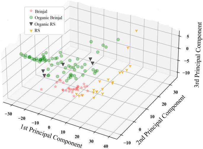
To reduce the issue of high dimensionality of hyperspectral data, we applied the Principal Component Transformation (PCT). This process resulted in transforming the high dimensional reflectance data to a manageable dimension of 35 while retaining the gross spectral features of full dimensional data. The first three PCA components explained 80% of variances, and all 35 components explained nearly 99% of total variance. Fig. 3 shows the first three principal components in a 3-dimensional space of spectral reflectance data of the crops grown under organic and conventional cultivation practices.

The first three principal components of organic vs. conventionally cultivated crops in three-dimensional space (RS: red spinach).
Spectral discriminant analysis using statistical and machine learning approaches
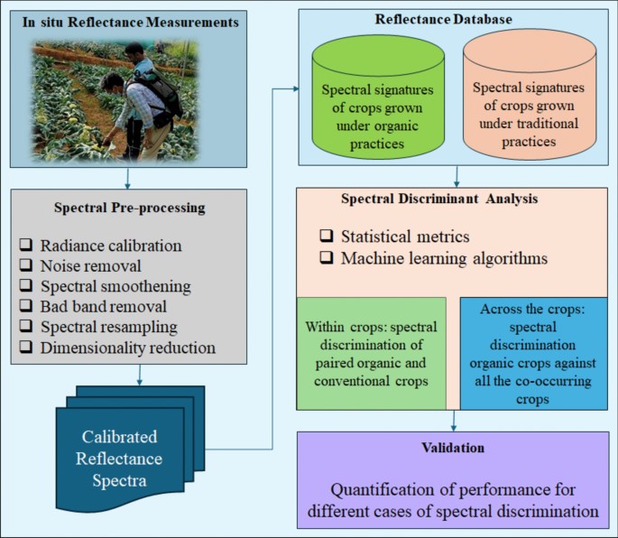
The methodological framework employed to discriminate various crop spectral signatures using statistical and machine learning algorithms is depicted in Fig. 4.

The methodological framework adopted for the spectral discrimination of organic and conventionally cultivated crops.
Two crops; – brinjal and red spinach, were cultivated under both organic and conventional agricultural practices. In contrast to the statistical separability approach utilized in previous studies, our evaluation of crop discrimination was conducted from a functional perspective. Specifically, we view it as a classification task where the quality of spectral discrimination is directly linked to classification accuracy. Moreover, a method selected for classification significantly impacts the accuracy of the results. Consequently, twelve distinct statistical and machine learning (ML) algorithms were employed for classification. We provide a brief description of the algorithms and the heuristics of tuning parameters for quick reference. Since these algorithms are widely reported, we recommend referring to the references cited for more details.
Logistic regression20,21 is a statistical modeling technique used for classification. A multiclass classification problem uses the one vs. rest (OvR) technique in which one by one class is targeted as a positive class, and the rest of the classes, as combined, are treated as a negative class. We used the ‘L2’ penalty because the resulting model is not sparing, and all the coefficients are reduced with the same factor. The utilized loss function for this algorithm can be expressed using Eq. (1):
$$\begin- Log loss = _ – y\log (y’) – (1-y)\log (1-y’), \end\sum _c$$
(1)
where (x, y) \(\in\) D is the spectral reflectance dataset, y is the actual labels of the crop classes, and y’ is the predictions by the trained logistic regression model.
Ridge classifier22 applied to the crop spectral reflectance dataset converts all the class labels to be within the range of -1, +1 and then solves the crop discrimination problem as a regression task. The regularization strength (alpha) values are 1.0 for this problem. ‘L2’ penalty is added to the loss function in ridge classification, which can be seen in Eq. (2):
$$\begin Loss = \sum _^n (y_i – (w_i x_i + c))^2 + \lambda \sum _p_1-p_2^n w_i^2, \end$$
(2)
where \(\lambda\) is the regularization parameter used for large coefficient values, w is the parameters vector, c is the intercept, and (x, y) belongs to the utilized dataset, x is the feature vector, and y is the class label.
Stochastic gradient descent (SGD)23 classifier implements the regularized linear model with SGD optimization. The loss gradient is calculated for every spectral reflectance sample at a time and updated in the model. It allows small batch learning, and convex loss function ‘hinge’ loss is used, expressed in expression (3):
$$\begin{aligned} L(y_i, f(x_i)) = max(0, 1 – y_i.f(x_i)), \end{aligned}$$
(3)
where \(y_i\) is the actual label and f(\(x_i\)) is the output label function.
K-nearest neighbor (KNN)24 is the simple but elegant classification algorithm in which a classification decision is based on the nearest neighbor value ‘k.’ A targeted data point measures Euclidean distance, and the point is classified based on the majority voting. The value of ‘k’ can only be an odd positive number. The Euclidean distance can be calculated using the below-given formula in Eq. (4):
$$\begin{aligned} D(v_1, v_2) = \sqrt{\frac{\sum _{i=1}^M (x_i – y_i)^2}{d}}, \end{aligned}$$
(4)
where \(v_1\)= (\(x_1\),\(x_2\),\(x_3\ldots x_d\)) and \(v_2\)= (\(y_1\),\(y_2\),\(y_3\ldots y_d\)) are the feature vectors, and M is the feature space dimensionality.
Decision tree classifier25 is a supervised, non-parametric algorithm to solve a classification problem. It uses different algorithms to decide on splitting the nodes’ hierarchy. We used the ‘Gini’ algorithm for this crop discrimination problem. Gini impurity can be calculated based on Eq. (5):
$$\begin{aligned} Gini_{node} = \sum _{i=1}^n P_i (1-P_i), \end{aligned}$$
(5)
where \(p_i\) is the probability of picking a data point from utilized spectral dataset classes, and n is the total number of classes.
Support vector machine (SVM)34 is one of the most sophisticated classifiers used for classification purposes. SVM tries to draw a hyperplane between the classes and maximize the margins. Primarily, SVM is a binary classifier using multiple SVM machines; it can also be applied to multiclass problems. We used a linear kernel for our crop spectral reflectance discrimination problem. Equation (6) gives the hyperplane equation:
$$\begin{aligned} W.x + b = 0, \end{aligned}$$
(6)
where W is the average vector to the hyperplane, x is the input data vector, and d is the intersection of the hyperplane from the origin.
Crop spectral reflectance data can be non-linearly separable, SVM with radial basis function (RBF) kernel can be used. RBF tries to find the similarity between two points, \(p_1\) and \(p_2\). Equation (7) can represent the RBF kernel:
$$\begin{aligned} K(p_1, p_2) = e^\frac{-||p_1-p_2||}{2\sigma ^2}, \end{aligned}$$
(7)
where \(\sigma\) is the variance, \(||p_1-p_2 ||\) is the Euclidean distance between the points \(p_1\) and \(p_2\).
Gaussian naïve Bayes26 algorithm primarily works based on the Bayes theorem and supposes that each class in the crop spectral reflectance dataset follows the normal distribution. The Gaussian NB considers features independent of each other; hence, the covariance matrix will be diagonal. The Gaussian’s naïve Bayes theorem can be expressed as the following Eq. (8):
$$\begin{aligned} P(x|y = c) = \frac{1}{2\pi ^\frac{d}{2}\sqrt{|\sum _c|}}.e^{-(x-\mu _c)^T\sum _{c}^{-1}(x-\mu _c)}, \end{aligned}$$
(8)
where \(P(x_i|y=c)\) is the posterior probability for a class c, d is the dimension of \(x, \sigma _c\) is the covariance matrix, \(\mu _c\) Is the mean for a class c.
Adaboost24,27 is an adaptive ensemble learning algorithm that combines many weak classifiers to form a robust classifier and tweaks the weak classifiers to perform best based on previous iterations. Adaboost gives more weight to minor discriminative instances and more weight to easily discriminatory examples. In general, a boosted classifier can be expressed as shown in Eq. (9):
$$\begin{aligned} F_K(x) = \sum _{k=1}^K f_k(x), \end{aligned}$$
(9)
where x is an object given as an input in weak learner \(f_k\) and returns the output as an object of the class, and K is the total number of classifiers in the boosting algorithm.
Random forest28 is an ensemble learning technique combining multiple decision trees for classification. The crop spectral reflectance dataset is classified based on the majority voting for a particular class. We considered 100 decision trees as estimators. Variable importance is measured by the dataset \(D = [{(X_i, Y_i)}]_(i=1)^n\) before fitting it with random forest decision trees.
Gradient boosting29 algorithm is also an ensemble learning technique used for supervised classification. It includes decision trees as weak learners. Combined, it uses several weak learners and makes a single strong learner iteratively. It tries to minimize the mean squared error as given in Eq. (10):
$$\begin{aligned} MSE = \frac{1}{n} \sum _i(\hat{y} – y_i)^2, \end{aligned}$$
(10)
where n is the number of training samples in the reflectance spectral dataset, \(\hat{y}\) are the predicted values of the function \(\hat{y} = F(x), y_i\) is the actual class label value.
Quadratic Discriminant Analysis (QDA)30 is a generative classifier that presupposes data following the normal distribution. QDA is suitable for datasets in which classes are not linearly discriminative. The discriminative boundary is non-linear in the case of QDA. The covariance matrix is not the same for each category in the case of QDA. The discriminative function of QDA can be expressed as given in Eq. (11):
$$\begin{aligned} \delta _n(x) = -\frac{1}{2} \log |\sum _n| – \frac{1}{2}(x-\mu _n)^T \sum _n^{-1}(x-\mu _n) + \log \pi _n, \end{aligned}$$
(11)
where \(\Sigma _{n}\) is the covariance matrix, which is different for every class, \(\mu _n\) is the mean of a class.
Validation
We evaluated the performance of the discriminant analysis by the stratified five-fold cross-validation method with a 7:3 training and validation split ratio. While splitting the dataset, the shuffle was on, and the random state was initialized with 11 for each fold’s iteration. Hyperparameters were fixed before the training for all models. We assessed the models’ performance utilizing several widely referred non-parametric validation metrics. These metrics provide valuable insights into various aspects of the discrimination performance, such as Accuracy, Precision, Recall, F1 score, Mean Squared Error, Receiver Operating Characteristic (ROC), and Area Under the curve (AUC)31. Using this rigorous evaluation framework, we validated the reliability and robustness of the results. All the analysis is performed using Python and the Sklearn library.
Accuracy, precision, recall, F1 score, and mean squared error are essential metrics used to evaluate the performance of classification models, particularly in the context of imbalanced data sets such as crop labelling tasks. Accuracy represents the proportion of correctly predicted crop labels out of the total labels, providing a general measure of overall correctness. Precision for a specific crop class measures the ratio of correctly predicted labels for that class to the total predicted labels for that class, highlighting the model’s ability to avoid false positives. Recall for a particular crop class indicates the ratio of correctly predicted labels for that class to the total correct and incorrect labels for that class, showcasing the model’s ability to identify all relevant instances of that class. The F1 score, the harmonic mean of precision and recall, provides a balanced measure of a model’s performance, especially in imbalanced datasets where the classes have unequal distributions. It helps in determining the classification quality, considering both false positives and false negatives. The mean squared error measures the average squared difference between predicted and actual labels, which helps to assess the trained model’s quality. In contrast with these numerical description-based validation metrics, the Receiver Operating Characteristic (ROC) curve is a graphical representation that illustrates the performance of a crop classification model across various thresholds. It provides valuable insights into the trade-off between the true positive rate (TPR) and the false positive rate (FPR) at different threshold values. The area under the ROC curve (AUC-ROC) is a commonly used metric to quantify the overall performance of a classification model. A higher AUC-ROC value indicates better discrimination capability, with a value of 1 indicating perfect classification and a value of 0.5 indicating random classification.
link


