Development and validation of machine learning models based on stacked generalization to predict psychosocial maladjustment in patients with acute myocardial infarction | BMC Psychiatry

Participants and data collection

A convenience sampling method was used to recruit young and middle-aged patients with AMI who were treated at the Departments of Cardiovascular Medicine of two tertiary hospitals (Center I and Center II) in Guangdong Province, China, from October 2021 to January 2024. Patients were required to fulfill the following inclusion criteria: (1) initial diagnosis of AMI according to the 2018 4th edition of the European Society of Cardiology ‘Guidelines for the Diagnosis and Treatment of Acute Myocardial Infarction’ [27]; (2) age 18–59 years [28]; (3) stable condition 1 month after discharge; (4) absence of mental illness; and (5) able to complete the designated questionnaires. Patients were excluded if they: (1) had severe damage to other vital organs (e.g. kidney, liver, lung) or other serious chronic diseases (e.g. malignant tumors); or (2) were participating in interventional studies that may affect psychological adjustment.

The process of data collection was divided into two stages. In the first stage, sociodemographic and disease-related variables, Perceived Stress Scale (PSS), Fear of Progression Questionnaire-Short Form (FoP-Q-SF), and Social Support Rating Scale (SSRS) data were collected before discharge. In the second stage, the PAIS-SR was used to assess psychosocial adjustment one month after discharge.

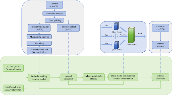
A total of 734 young and middle-aged patients diagnosed with AMI were enrolled in this study. Data from Center I (n = 458), designated the “internal dataset”, were randomly divided into an internal training set (n = 320) and an internal test set (n = 138). Data from Center II (n = 276), designated the “external dataset”, were employed for external validation of the model. A flowchart showing the study overview in Fig. 1.

This study was conducted in accordance with the Declaration of Helsinki and followed the Transparent Reporting Guidelines for Multivariate Predictive Models for Prognostic Studies (TRIPOD) [29] (Supplement 2).

The flowchart outlining the study overview. *Note: Participants from Center I were randomly divided into an internal training set and an internal test set. Six machine learning models were trained and optimized on the pre-processed training set using k-fold cross-validation and grid search. The internal test set was used for internal validation of the models. Models with better internal training set performance were then used to construct a stacked generalization model architecture, which was further validated in internal test set. Participants from Center II were used as an external dataset to perform external validation on all the models

Variables and measures

After conducting a literature review, expert consultation, and discussion, the following potential predictors of psychosocial adjustment in patients with AMI were identified.

Sociodemographic and disease-related variables

Sociodemographic characteristics identified were: sex, age, education level, work status, smoking history, and alcohol consumption history. Disease-related characteristics included: underlying diseases, onset symptoms, disease classification, and Killip classification.

Other relevant influencing variables

Psychosocial adjustment

Psychosocial adjustment was assessed using the self-report version of the Psychosocial Adjustment to Illness Scale (PAIS-SR) developed by Derogatis et al. [30]. The Chinese version of PAIS-SR was translated and validated by Yao et al. [31] (Cronbach’s α = 0.87). The PAIS-SR contains 44 items and each item is scored using a four-point scale (i.e. 0–3). The total score range of the PAIS-SR is 0 to 132 points, higher scores are associated with psychosocial maladjustment. In this study, Cronbach’s α for the PAIS-SR was 0.90, and participants were categorized based on their adjustment levels into groups with low adjustment (0–50 points) and high maladjustment (51–132 points).

Perceived stress

Perceived stress was assessed using the Perceived Stress Scale (PSS) [32]. The PSS consists of 14 items, all of which are scored using a five-point Likert scale, with scores ranging from 0 for ‘never’ to 4 for ‘always’; total scores range from 0 to 56 points, with higher scores indicating greater levels of perceived stress. Total score ≥ 25 points indicates that an individual is experiencing health-threatening stress levels, while total score < 25 points indicates that the individual is not experiencing health-threatening stress levels [32]. The Cronbach’s α of PSS is 0.78 [32]. In this study, the Cronbach’s α of PSS was 0.87.

Fear of disease progression

Fear of disease progression was assessed using the Fear of Progression Questionnaire-Short Form (FoP-Q-SF) [33]. The FoP-Q-SF consists of 12 items, all scored using a five-point Likert scale, with scores ranging from 1 for ‘never’ to 5 for ‘always’. The total score of the FoP-Q-SF ranges from 12 to 60 points; higher scores indicate a more intense fear of disease progression. Total score ≥ 34 points indicates that the individual has psychological dysfunctional, while total score < 34 points indicates that an individual has normal psychological function. The Cronbach’s α of FoP-Q-SF is 0.86 [33]. In this study, the Cronbach’s α of FoP-Q-SF was 0.87.

Social support

Social support was assessed using the Social Support Rating Scale (SSRS) [34]. The SSRS comprises 10 items covering three dimensions: subjective support (n = 4), objective support (n = 3), and utilization of support (n = 3). Total score ranges from 12 to 66 points, with scores of 45–66, 23–44, and 12–22 points considered low, moderate, and high, respectively; higher scores indicate greater levels of social support. The Cronbach’s alpha of the SSRS is 0.87 [34]. In this study, Cronbach’s α for the SSRS was 0.73.

Data pre-processing

Data were cleaned using the Chi-square test to identify statistically significant features (P < 0.15). Multivariate analysis of the internal training set was used to identify important features (P < 0.05) among those determined to be statistically significant. All ML models were processed and visualized using Python 3.10 software, and data were analyzed using SPSS 21 software.

In this study, the unbiased ordinal features of patients were handled using one-hot encoding, biased ordinal features were processed with ordinal encoding, and continuous numerical features underwent normalization and standardization.

Model development

In this study, ML technology was used to develop a risk prediction model for psychosocial adjustment screening of young and middle-aged patients with AMI. The algorithm selection criteria were as follows: (1) the algorithm should be suitable for the data characteristics of this study and (2) the algorithm should save computing power and computing time. Considering the small sample size of the dataset and the large number of initial features, six ML algorithms were finally selected to train the initial model: logistic regression (LR), decision tree (DT), random forest (RF), extreme gradient boosting (XGBoost), support vector classification (SVC), and deep neural network (DNN) [35, 36].

The optimal hyperparameters of each model were determined in the training process by grid search combined with a greedy algorithm and the K-fold cross-validation (K = 5) method. First, the most influential hyperparameter of each model was searched within the parameter space by grid search. Once the optimal value was confirmed, the hyperparameter was assigned a value, and the tuning process moved on to search for and confirm the next most influential hyperparameter until all needed hyperparameters were assigned. The learning curve was used to test whether the model was overfitting or underfitting before and after model training. After the initial model was trained, the Stacked Generalization method was used to integrate the advantages of the model and construct the final prediction model.

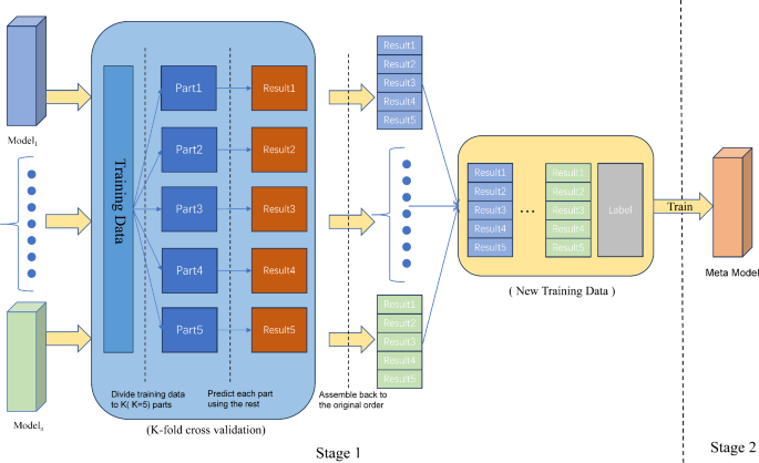
Stacked Generalization was applied with K-fold cross-validation (K = 5). The training process comprised two stages. In first stage, n base models were applied to internal training set using K-fold cross-validation. Then the prediction results of base models and labels of groundtruth were assembled to form a new training dataset. In the second stage, the meta model was trained using the new training dataset. The process of training is shown in Fig. 2.

The Stacked Generalization process. *Note: In first stage, n base models were applied to internal training set using K-fold cross-validation. Then the prediction results of base models and labels of groundtruth were assembled to form a new training dataset. In the second stage, the meta model was trained using the new training dataset

Stacked models are often superior to the best single models they contains, although their ability to perform well relies on inclusion of a mix of strong and diverse single models [26]. Therefore, in this study, base models to be stacked were selected based on the principle that each stacked model must achieve the best performance in at least one evaluation metric in the internal test set and by maximizing the differences in model architectures, to integrate the advantages of different model structures. LR commonly serves as the default choice of meta model; however, the performance of each selected model in the meta model was compared to determine the optimal choice of meta model for this study.

In some similar studies [37,38,39], all pre-trained models were engaged in the ensemble process. Therefore, to support the validity of the method of applying Stacked Generalization used in this study, trials were conducted to compare the performance of the model constructed with that of all pre-trained models, if not all pre-trained models were used in the model constructed in this study. All stacked models applied hyperparameters pre-confirmed during the grid search process.

Model validation

The model was validated using both internal test set and external dataset; the evaluation metrics included: Brier score, calibration slope, calibration intercept, area under the curve (AUC), specificity, sensitivity, negative predictive value (NPV), positive predictive value (PPV), Youden index, and accuracy [40]. After all models were fully trained on the internal training set, the external dataset and internal test set were used to test the generalization error of models. Decision curves were used to evaluate the clinical usefulness of the model for both the internal test set and the external dataset, while receiver operating characteristic (ROC) and calibration curves were used to evaluate the performance of models.

To verify the advantage of Stacked Generalization over other ensemble methods in avoiding overfitting, achieving higher accuracy, and offering flexibility, Soft Voting and Hard Voting were also applied in selected models. Soft Voting involves predicting the class label based on the weighted average of the probabilities output by individual models, while Hard Voting assigns the class label based on the majority vote of the individual models. The results of these methods were then compared to the performance of Stacked Generalization in comparative trials.

Model explainability

SHapley Additive exPlanations (SHAP) is a powerful framework based on cooperative game theory used for interpreting ML models, and provides a way to attribute the output of a model to its input features. By assigning each feature an importance value, SHAP helps to explain how individual features contribute to a model’s predictions. In this study, SHAP was applied to interpret the trained prediction model.

For other technical details, please refer to eMethods in Supplement 1.