Deep learning for robust orbit control of Elettra 2.0 storage ring

Closed orbit correction in Elettra 2.0
Our proposed method employs two models, a controller, and a system model, and is implemented using DCNN architecture. This section reviews the main concepts of CNNs and closed orbit correction in Elettra 2.0.
Elettra 2.0 storage ring is a low-emittance synchrotron light source under construction at Elettra Synchrotron Trieste, Italy. The Elettra 2.0 lattice consists of 12 cells, each containing instruments, namely two types of long dipoles (2 dipoles with 3.6° bending angle and 64 cm length and four dipoles with 6.5° bending angle and 80 cm length). The lattice has a natural emittance of 0.25 (nm.rad) and 259.2 (m) circumference25.
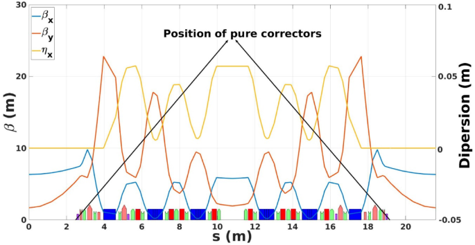
According to Table 1, the orbit control system of Elettra 2.0 consists of 24 pure correctors (two pure correctors per cell) and 168 beam position monitors (BPMs), with 14 BPMs in each cell distributed along the ring. Hereafter, we refer to a pure corrector as a kicker. The kickers are horizontal and vertical electromagnets that can adjust the trajectory of the electron beam through minor deflections. BPMs are used to measure the transverse position of an electron beam. They can detect the signals induced on electrodes or strip lines. The measured position can be positive or negative, with zero indicating that the beam is centered within the chamber. Also, each cell consists of 8 quadrupole electromagnetics (4 focusing and 4 defocusing) and 20 sextuples electromagnetics (some of the sextuplets have coils for correctors, and others create skew quadrupoles to control the coupling of the machine). Additionally, four combined multipoles (octupoles and pure correctors) per achromat reinforce the control of the tune shift with amplitude26. This layout is illustrated in Fig. 1

A cell sample in the Elettra 2.0 lattice which highlights crucial characteristics of the system. The blue and red lines indicate how particles move in the horizontal and vertical directions, while the yellow line shows how the arrangement of the lattice influences the particles’ paths.
Singular value decomposition (SVD) represents a conventional approach commonly employed in orbit correction27. The iterative SVD method involves applying SVD to BPM data to estimate kicker magnet strengths. SVD facilitates the decomposition of the BPM data matrix into singular vectors and values and identifies dominant modes of variation. The iterative refinement of this process allows for the extraction of kicker magnet strengths corresponding to specific beam positions. The main advantage of the iterative SVD method is its transparency and interpretability, allowing for direct physical insights from the decomposition results, which enhance the understanding of beam dynamics. However, it is noteworthy that SVD may face challenges in handling highly nonlinear relationships and may not capture subtle dependencies in the data as effectively as ML methods. A real-world synchrotron is a complex environment with inherent non-linearities arising from sextupole magnets, magnetic field imperfections, and potential coupling effects. While SVD offers excellent performance, these non-linearities can limit the ultimate achievable stability. Our primary motivation for exploring a machine learning approach was to develop a data-driven model that can capture these complex, non-linear dynamics without requiring an explicit analytical model.
Control systems
Control systems is an area of study focusing on dynamic systems and their associated feedback mechanisms. They can regulate various parameters, such as temperature, speed, and population. They can be open-loop or closed-loop, depending on whether they use feedback. Closed-loop systems have better performance but are more complex. Control systems have many applications in different fields, such as aerospace, robotics, power systems, and biomedical engineering. They can also be integrated into other technologies, such as sensing, communication, and decision-making, to create clever and intelligent systems. Control systems are an active and interdisciplinary research area with many topics and challenges, such as nonlinear and adaptive control, optimal and stochastic control, distributed and networked control, learning and data-driven control, and resilient and safe control. Control systems research aims to develop new theories, methods, and tools for modern future systems28,29,30.
Neural controller
Intelligent neural controllers are intelligent control techniques that use artificial neural networks (ANNs) to model, design, optimize, and tune closed-loop control systems (CLCS). CLCS uses sensor feedback to adjust the control variables of a process or a system in real time. ANNs are computational models that can learn from data and approximate complex nonlinear functions. Intelligent neural controllers can improve the performance and reliability of CLCS, especially for multivariable and nonlinear processes that are difficult to control by conventional methods. Intelligent neural controllers can also adapt to changing environments and disturbances and predict future states of the system using machine learning methods31,32,33.
Our study considered the synchrotron system and the kicker controller to measure the controller’s effect on BPMs. As highlighted in the introduction, only a few studies have been conducted in this field13,19. Neural networks are powerful universal function approximators, making them ideally suited for learning the intricate relationships between magnet errors, beam position monitor (BPM) readings, and the required corrector magnet strengths.
Deep convolutional neural network
DCNN is an artificial neural network that can learn from data and extract features using multiple layers of filters and nonlinear activations. It can handle high-dimensional and spatially correlated data, such as images or signals, and achieve high accuracy and generalization. It uses a combination of convolutional, pooling, and fully connected layers to automatically and adaptively learn spatial hierarchies of features from the input data. That allows it to identify complex patterns within data, making it more effective at handling high-dimensional data and large datasets. Convolutional neural networks can learn features invariant to transformations, exploit the local structure and correlation of the data, and have fewer parameters and better generalization than multilayer perceptron (MLP). MLP treats each input as independent and does not consider their spatial or temporal relationships34,35. Furthermore, fine-tuning is a common technique used in transfer learning, particularly with DCNNs36,37,38,39,40.
Materials and methods
Our machine learning pipeline begins with data collection, during which we shall utilize the ELEGANT (ELEctron Generation ANd Tracking) code to create a comprehensive dataset of beam dynamics. The raw data will then be preprocessed and transformed into a format suitable for model training.
Next, we shall train a system model to understand the underlying dynamics of the beam, which forms the foundation of our control strategy. In parallel, we aim to develop a controller model to predict the optimal kicker magnetic field strength needed for beam correction. Finally, we intend to fine-tune the controller model to enhance performance and adapt it to specific operational conditions. Additionally, we use the ADAM optimizer for training, which efficiently handles complex optimization tasks.
In these models, the input layer consists of a one-dimensional vector length N. The hidden layer includes convolutional blocks, each with a convolutional layer, a batch normalization layer, a rectified linear unit (ReLU) activation function, and a max pooling layer. The convolutional layer applies filters to the input vector and produces a feature map. The batch normalization layer normalizes the feature map and improves the stability and speed of training. The ReLU activation function introduces nonlinearity and sparsity to the feature map. The max pooling layer reduces the dimensionality and noise of the feature map by selecting the maximum value in each region. The output layer is a fully connected layer that maps the final feature map to a one-dimensional vector of length M.
We aim to assess the performance of the trained system model using two primary metrics: mean squared error (MSE) and normalized mean absolute error (NMAE). The MSE quantifies the average squared difference between the predicted values and the actual values for the kickers. On the other hand, the NMAE will be calculated by dividing the mean absolute error (MAE) by the range of the observed values, which normalizes the error to a scale between 0 and 1. A lower NMAE indicates a better alignment between the predicted and actual values, while a higher NMAE reflects a poorer correspondence. We may also express NMAE as a percentage for a more straightforward interpretation.
Additionally, we shall evaluate the controllers based on the steady-state error, a crucial performance metric in control systems. Maintaining the beam centered in the chamber as far as possible in a synchrotron is vital for optimal operation.
We used Python language and the Keras library, which has a TensorFlow backend, to implement the proposed method.
Data collection and preprocessing
Since Elettra 2.0 is still in the design and construction stage, we used the simulation data as input for the ML procedure. The disturbed beam was simulated using the ELEGANT code, which uses several thousand machine ensembles41. Table 2 shows that the magnet’s errors disturbed the beam in our simulation42. This should be considered in the future when other sources of errors are considered.
ELEGANT applied errors and disturbed the beam. The position of the disturbed beam—which remained viable for correction—can be determined in simulation using the SVD method using BPM. The SDDS (self-describing data sets) output files from ELEGANT contain all these simulated outcomes. Therefore, we converted the SDDS files and extracted the fields as illustrated in Table 3 during preprocessing to obtain the final cleaned data, originating entirely from the complete simulation process, which has 360 columns as attributes.
The dataset comprises approximately 9,500 unique machine ensembles. For each ensemble, we introduced a realistic distribution of magnet errors, including misalignments, tilts, and fractional strength errors, as detailed in Table 2. This created a statistically representative set of “disturbed” initial closed orbits. For each disturbed orbit, we simulated an 11-step iterative correction process using the conventional SVD method. The final dataset consists of the full sequence for each ensemble. The process iteratively refines the beam state, where at each step the controller calculates a new set of absolute kicker strengths that replaces the previous configuration. This sequence continues until the beam converges after 11 steps. Table 4 illustrates the sequence of correction steps:
We divided the dataset into training (72%; ~ 6800 samples), validation (18%; ~ 1700 samples), and a held-out test set (10%; ~ 1000 samples). The validation set served to monitor overfitting during the training process. The final reported performance metrics were evaluated only on the test set, which the model had not previously encountered.
To provide a clear performance baseline, it is critical to quantify this initial disturbance. Across the unseen test data, the average absolute deviation of this initial ‘Uncorrected Beam’ was 650.85 µm, with a standard deviation of 258.67 µm. This value establishes the scale of the orbit correction challenge that both the conventional SVD method and our proposed DCNN controller must address. The following sections will detail the performance of each method in correcting this initial deviation.
In our work, we exclusively utilized beam position data for the machine learning procedure, a decision grounded in several key considerations. First, BPMs provide direct and high-resolution measurements of beam positional deviations, effectively capturing the cumulative effects of all disturbances and errors in the beam path. Focusing on these observable outcomes allowed us to address the immediate state of the beam that requires correction. Moreover, limiting our input features to beam position data could simplify the model, enhance computational efficiency, and reduce the risk of overfitting without compromising the model’s ability to learn the necessary correction patterns.
Additionally, the influences of other potential error sources, such as fluctuations in radio frequency components or misalignments in dipole, quadrupole, and sextupole magnets, are implicitly embedded within the BPM readings. This indirect inclusion ensures that the model accounts for these factors without additional complex and potentially redundant data inputs. By concentrating on beam position data, we can enhance the generalizability of our model, enabling it to perform effectively across varying operational conditions. This feature engineering approach streamlines data preprocessing and model training and ensures that the model remains robust and focused on the primary objective of the beam trajectory correction.
Model training and architecture
The choice of a Deep Convolutional Neural Network (DCNN) over other architectures, such as a standard Multi-Layer Perceptron (MLP), is critical and stems directly from the physical layout of the accelerator. As the Elettra 2.0 ring contains 168 BPMs distributed spatially around its 259.2-m circumference, these sensors are not independent. A localized orbit distortion (a “bump”) caused by a specific error source creates a characteristic, spatially correlated pattern across adjacent BPMs. DCNNs are explicitly designed to exploit this spatial locality by treating the BPM readings as a 1D signal. Deeper layers integrate these features to detect increasingly intricate, global orbit forms, while the convolutional filters learn to identify local distortion patterns. By treating each BPM input separately, an MLP would lose this important spatial information and need a lot more parameters to learn the same correlations. We also attempted an MLP architecture but found it underperformed due to higher parameter counts and challenges in training with our dataset size, reinforcing the choice of DCNN for exploiting spatial correlations.
Each model was trained separately using a batch size of 16 and 50 epochs. They were all implemented in Python using the Keras package and a TensorFlow backend (Training took approximately 2 h on a Colab T4 GPU; inference: 125 µs/evaluation orbit). A MinMaxScaler was used to scale the input data to [0,1] range separately per device type (BPMs/kickers). We used the ADAM optimizer for optimization, minimizing the Mean Squared Error (MSE) as the loss function and maintaining a constant learning rate of 0.001.
The DCNN architecture for both models is built from a series of convolutional blocks. Each block contains a Conv1D layer to extract spatial features, a batch normalization layer for stable and fast training, and a ReLU activation function to introduce non-linearity. This process serves a dual role. It improves computational efficiency by reducing dimensionality while also refining the model’s focus by isolating the peaks of the orbit distortion. By selectively propagating only these significant deviation signals, the layer creates a more compact and robust representation of the beam state.
Implementation details of system model
The system model uses uncorrected beam data and kicker magnet strengths as inputs to forecast corrected beam positions. It leverages a deep convolutional neural network to predict optimal beam corrections.
This model serves two distinct purposes: first, it evaluates the performance of the designed controller outputs in a simulated synchrotron environment; second, it provides a reference point for transfer learning in fine-tuning the controller model.
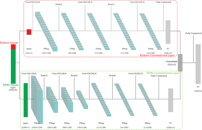
This section aims to process and integrate diverse input types effectively. To accommodate this, we incorporated “multi-sensor data fusion” into the model architecture43,44. Specifically, we designed separate convolutional blocks for kickers and BPMs, allowing the model to process and integrate the distinct sensor data streams effectively. Figure 2 illustrates the implementation details of DCNN in the system model’s architecture. The convolutional layers, pooling layers size, feature map shapes are shown on it.

Implementation details of DCNN in the system model’s architecture.
Implementation details of controller model
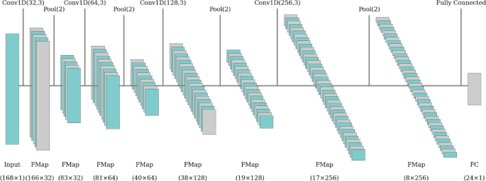
The uncorrected beam data is used as input for the ML algorithm. Our ML approach employs a DCNN model similar to the system model, which predicts the optimal strength values of the kicker magnetic fields based on the uncorrected beam positions. Figure 3 illustrates the implementation details of the DCNN in the controller model’s architecture. It is important to note that the controller is trained to output the full, absolute strength value for each of the 24 kickers, not an incremental (delta) change from the previous state.

Implementation details of DCNN in the controller model’s architecture.
Fine tuning in controller model
To further improve the controller model’s performance and ensure that it accurately predicts the optimal kicker strengths for beam correction, we implemented a fine-tuning strategy as a transfer learning approach, utilizing the pre-trained system model as a fixed simulator of beam dynamics. During fine-tuning, the parameters of the system model were kept unchanged; that is, we did not update its weights during backpropagation. This ensures that the system model continues accurately representing the established beam dynamics, and any adjustments during training are made solely within the controller model. The target outputs for the system model were set to the desired reference beam positions, representing an ideally corrected beam state.
We obtained an error signal that reflects how well the predicted kicker strengths achieved the desired correction by computing the loss between the system model’s output (the simulated corrected beam positions) and the desired reference positions. This error was then backpropagated only through the controller model, updating its weights to minimize the discrepancy. Through this fine-tuning process, the controller model learns to produce kicker strength predictions that, when applied, result in beam positions closer to the desired reference, thereby effectively improving the accuracy and robustness of the beam correction strategy.
link


