
Deep learning driven interpretable and informed decision making model for brain tumour prediction using explainable AI

Brain Tumour diagnosis presents a unique set of challenges, including the need to handle noisy and sparse datasets, ensure reliable and accurate predictions, and provide interpretable outputs for clinical decision-making. Traditional models often fall short in addressing these issues, struggling with scalability, over-reliance on intensity-based features, and a lack of transparency in their predictions. These limitations not only hinder diagnostic precision but also reduce trust and usability in critical medical environments. To overcome these challenges, the proposed model introduces a transformative approach that combines advanced deep learning techniques, robust data augmentation, and explainable artificial intelligence (XAI) to deliver a reliable, interpretable, and adaptable solution for brain tumour diagnosis. The overview of the proposed model is given in Fig. 1.
Figure 1 presents an advanced, integrated system for brain tumour diagnosis, leveraging data collection from diverse sources such as hospitals, mobile medical devices, patients, and satellites, all connected through the Internet of Medical Things (IoMT). The collected imaging data is processed through three key stages: pre-processing (enhancing and preparing data), processing (analyzing data using advanced deep learning models), and post-processing (refining results for clinical interpretation and interpretability using XAI). These post-processing outcomes are then sent to cloud computing, which ensures efficient storage, analysis, and real-time accessibility, enabling scalability and collaboration among medical professionals. The model then culminates in a validation phase to ensure the accuracy and reliability of predictions, providing a streamlined, scalable, and precise solution for modern medical imaging workflows.
Figure 2 presents a comprehensive framework for brain tumour diagnosis, emphasizing the pivotal role of cloud computing in enabling efficient data management and real-time collaboration. The system begins with a robust Brain Tumour Data Collection System, gathering medical imaging data from diverse sources such as hospitals, healthcare mobile devices, and satellites, all interconnected via the IoMT. The collected data is routed to cloud-based servers, ensuring centralized storage and facilitating secure, real-time accessibility for healthcare professionals.
The data undergoes three key processing layers within the cloud infrastructure: Data Pre-Processing, where raw data is cleaned and enhanced for analysis; Data Processing, which employs advanced AI and deep learning techniques to detect potential brain tumours; and Data Post-Processing, which focuses on interpretability and providing transparency in decision making using XAI. These interpretable outcomes remain in the cloud, enabling scalable storage and seamless access for healthcare teams. The cloud system also facilitates scalability, allowing the storage and processing of vast amounts of medical imaging data without compromising performance or reliability.

Overview of the proposed interpretable brain tumour prediction model.

Abstraction of the proposed interpretable brain tumour prediction model.
Once the data is available in the cloud, it is made accessible through advanced Visualization Tools, which transform the processed information into clear and interpretable formats. These tools allow clinicians to quickly understand the results and make informed decisions. The visualization ensures that whether a Brain Tumour is detected or not, the results are presented in an easy-to-interpret and validated manner. This flow, from post-processing to cloud integration and visualization, highlights the system’s ability to streamline workflows and improve diagnostic accuracy in modern medical imaging. This flow, from post-processing to cloud integration and visualization, highlights the system’s ability to streamline workflows and improve interpretable diagnostic accuracy in modern medical imaging.

Proposed interpretable brain tumour prediction model.
Figure 3 shows the proposed interpretable model for brain tumour prediction, which is structured into eight distinct steps as outlined below.
Brain tumour data collection
The proposed model begins with the collection of a dataset36 obtained from brain images. High-quality and correct image data is very important at this stage since any errors in this stage may render the other stages erroneous. The collected images are then sent to the preprocessing layer for further changes and data preparation.
Preprocessing layer
The collected data undergoes a systematic preprocessing pipeline to ensure it is clean, consistent, and suitable for analysis. All MRI images were resized to standardized dimensions according to the input requirements of the respective deep-learning architectures used in the study. Pixel intensities were normalized to a [0, 1] scale using a rescaling factor of 1./255. Real-time data augmentation was applied during model training using Keras’ ImageDataGenerator. Techniques included rotations, shifts, zooming, shearing, and horizontal flips. These operations improved training diversity and contributed to more stable validation performance.
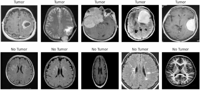
Sample Images from Dataset (Tumour and No Tumour)36.
Figure 4 shows images from the dataset, categorized into “Tumour” and “No Tumour” classes. These images involve image resizing, where all images are standardized to a uniform dimension of pixels. This ensures that the images are compatible with the deep learning model and reduces computational complexity.

Pixel Value Distribution (Tumour Images).

Class Distribution (Training and Validation Sets).
Figure 5 shows a pixel normalization is performed by scaling the pixel values to a range of [0, 1]. This step enhances the model’s convergence speed and stability during training. The histogram in this figure highlights any patterns, irregularities, or noise in the intensity values, allowing for a deeper understanding of the dataset’s properties.
Figure 6 shows the class distribution across training and validation datasets for the “Tumour” and “No Tumour” categories. This analysis is crucial to ensure that there is no significant class imbalance, which could introduce bias into the model’s predictions. A well-balanced dataset ensures a fair representation of both classes during training and testing.
Figure 7 displays sample augmented images with their corresponding labels (“Tumour” or “No Tumour”). Data augmentation is performed using techniques such as random rotations, shifts, zooms, and flips. This step significantly increases the dataset’s diversity, enabling the deep learning model to generalize better by exposing it to varied scenarios during training.
Figure 8 demonstrates the results of dimensionality reduction techniques such as t-SNE and PCA. These methods project high-dimensional data, revealing the clustering and separability between “Tumour” and “No Tumour” classes. This visualization aids in understanding how distinct the two classes are in the feature space, which can directly impact the model’s performance.
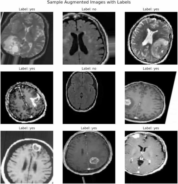
Sample Augmented Images with Labels.

t-SNE and PCA Visualization.

Figure 9 provides HSV color histograms for the dataset. These histograms analyze the color properties in the HSV (hue, saturation, and value) space, revealing variations and potential inconsistencies in the dataset. Understanding these properties can assist in refining preprocessing methods and ensuring uniformity across the dataset.

Random Image Samples with Labels.
Figure 10 presents a montage of randomly sampled images from the dataset, along with their labels (“Tumour” or “No Tumour”). This step serves as a final quality check, allowing researchers to visually confirm the diversity and correctness of the data after preprocessing.
Figure 11 overlays the pixel intensity distributions for “Tumour” and “No Tumour” images. This comparative histogram highlights distinct patterns and overlaps between the two classes, providing insights into how these differences might influence the deep learning model’s ability to distinguish between them.
After preprocessing is completed, the data is divided into two sets: 70% is allocated for training the deep learning model, while the remaining 30% is reserved for testing in the cloud database. This split ensures that the model learns from one dataset while being validated on another, unbiased set, thereby enhancing its generalization capabilities and reliability.

Pixel Intensity Distribution Comparison (Tumour vs. No Tumour).
Deep learning
The deep learning phase plays a vital role in the proposed system, dedicated to training the model to classify brain images into “Tumour” and “No Tumour” categories. A comprehensive evaluation of multiple state-of-the-art deep learning algorithms was conducted, including CNN, VGG16, ResNet50, EfficientNetB3, DenseNet121, Xception, and NASNet Large. Among these, NASNet Large outperformed the others, demonstrating superior accuracy and an unparalleled ability to automatically optimize its architecture for the given dataset.
NASNet Large relies heavily on convolutional operations to extract features from the input images. Convolution is defined as:
$$f_{{i,j,k}} = \sum\limits_{{m = 1}}^{M} {\sum\limits_{{n = 1}}^{N} {\sum\limits_{{l = 1}}^{L} {I_{i} + m,j + n,l.W_{{m,n,k,l}} + b_{k} } } }$$
(1)
Here, \({f}_{i,j,k}\) represents the value of the output feature map at position \((i,j)\) for filter \(k\). This value is computed by summing over all channels, where \({I}_{i}+m,j+n,l\) is the pixel value at position \((i+m,j+n)\) in channel \(l\) of the input image. The weights of the filter, denoted as \({W}_{m,n,k,l}\) determine how much each pixel contributes to the feature map. The \({b}_{k}\) term represents the bias for filter \(k\), which allows flexibility in the filter’s response. The size of the filter is defined by \(M\) (height) and \(N\) (width), while \(L\) indicates the number of channels in the input image. This operation helps the model detect patterns such as edges and textures critical for classification.
NASNet Large enhances computational efficiency by utilizing depthwise separable convolutions, which decompose the standard convolution into two steps: depthwise and pointwise convolutions. The operation is represented as:
$$f_{{i,j,k}} = \sum\limits_{{l = 1}}^{L} {\left( {\sum\limits_{{m = 1}}^{M} {\sum\limits_{{n = 1}}^{N} {I_{i} + m,j + n,l.W_{{m,n,l}}^{{depth}} } } } \right)} .\;W_{{l,k}}^{{point}} + b_{k}$$
(2)
Here, \({f}_{i,j,k}\) is the final output feature map at position \((i,j)\) for filter \(k\). First, the depthwise convolution is performed, where \({W}_{m,n,l}^{depth}\) denotes the weights applied to channel \(l\) of the input image, allowing each channel to be filtered independently. This is followed by the pointwise convolution, where \({W}_{l,k}^{point}\) combines the outputs across channels into a single feature map. The bias term \({b}_{k}\) adds flexibility to the filter’s output. By separating the operations, the computational complexity is reduced from \(O(M\times\:N\times\:L\times\:K)\) to \(O(M\times\:N\times\:L+L\times\:K)\), where \(M\) and \(N\) are the filter dimensions, \(L\) is the number of input channels, and \(K\) is the number of output filters.
NASNet Large is designed using Neural Architecture Search, which optimizes the network’s architecture by minimizing validation errors. The search process is formalized as:
$${A}^{*}=arg\underset{A\in\:\mathcal{A}}{{min}}E\left(A\right)$$
(3)
In this formulation, \(a\) represents a candidate architecture from the search space \(\mathcal{A}\), which is a set of all possible combinations of operations (such as convolutions, pooling, and identity mappings). The function \(E\left(A\right)\) denotes the validation error associated with a specific architecture \(A\), which measures its performance on unseen data. The optimal architecture \({A}^{*}\) is the one that minimizes the validation error, ensuring the best configuration for the task. This search is performed using reinforcement learning, where the performance of candidate architectures guides the exploration of \(\mathcal{A}\).
NASNet Large incorporates auxiliary classifiers to stabilize training and combat vanishing gradients in deeper layers. The total loss is computed as:
$${L}_{total}={L}_{main}+\alpha\:.{L}_{aux}$$
(4)
Here, \({L}_{total}\) is the combined loss used during training. \({L}_{main}\) represents the cross-entropy loss from the primary output layer, which measures the difference between predicted and true class probabilities. \({L}_{aux}\) is the auxiliary loss computed from intermediate layers of the network, ensuring that gradients flow effectively through all layers. The term \(\alpha\:\) is a weighting factor that determines the contribution of the auxiliary loss to the total loss. By incorporating \({L}_{aux}\), the network achieves better convergence and stability during training.
The final layer in NASNet Large uses a softmax activation function to predict class probabilities. The probability of an input xx belonging to class ii is given by:
$$P\left(y=i|x\right)=\frac{{e}^{{z}_{i}}}{\sum\:_{j=1}^{C}{e}^{{z}_{j}}}$$
(5)
In this equation, \(P\left(y=i|x\right)\) is the predicted probability for class \(i\), where \({z}_{i}\) represents the raw logit score for class \(i\) computed by the final dense layer. The denominator, \(\sum\:_{j=1}^{C}{e}^{{z}_{j}}\), ensures that the probabilities sum to 1 across all classes \(C\). For this binary classification task, \(C=2\), corresponding to “Tumour” and “No Tumour.” The class with the highest probability is chosen as the predicted label, allowing the model to output interpretable and confident classifications.
Once trained, the NASNet Large model was finalized as the proposed solution and advanced to the prediction phase for performance evaluation.
Predictions
In the prediction phase, the trained NASNet Large model evaluates its ability to generalize the patterns it had learned during training. These predictions are used to ensure a comprehensive evaluation. However, the NASNet Large model’s performance was considered satisfactory, allowing the system to proceed to the next phase: Explainable Artificial Intelligence (XAI).
Explainable artificial intelligence (XAI)
To make the model’s decisions transparent and interpretable, Explainable Artificial Intelligence (XAI) techniques are applied to the predictions generated by the NASNet Large model. In this case, LIME (Local Interpretable Model-agnostic Explanations) and Grad-CAM (Gradient-weighted Class Activation Mapping) were employed as the XAI approaches.
-
LIME: This technique explains individual predictions by perturbing the input data and observing the impact on the model’s output. It identifies the key features of the brain image that contributed most to the classification decision (e.g., specific pixel regions associated with Tumour detection). It approximates the original complex model \(\left(f\right)\) with a simpler surrogate model \(\left(g\right)\) in the local neighborhood of the instance being explained. The surrogate model is optimized as follows:
$$g=arg\underset{g\in\:G}{{min}}\sum\:_{{x}^{{\prime\:}}\in\:D}{\pi\:}_{x}\left({x}^{{\prime\:}}\right).{(f\left({x}^{{\prime\:}}\right)-g({x}^{{\prime\:}}\left)\right)}^{2}+\varOmega\:\left(g\right)$$
(6)
-
Here, \(g\) is the interpretable surrogate model, \(f\left({x}^{{\prime\:}}\right)\:\)is the output of the original model for a perturbed instance \({x}^{{\prime\:}}\). \(D\) is the perturbed dataset generated around the input instance \(x{\pi\:}_{x}\left({x}^{{\prime\:}}\right)\). is a proximity measure, often a kernel function, that assigns higher weights to perturbed instances \({x}^{{\prime\:}}\) closer to \(x\). For example:
$${\pi\:}_{x}\left({x}^{{\prime\:}}\right)=\text{e}\text{x}\text{p}(-\frac{{distance\:(x,{x}^{{\prime\:}})}^{2}}{{\sigma\:}^{2}})$$
(7)
-
\(\varOmega\:\left(g\right)\) is a regularization term to enforce simplicity in the surrogate model \(g\). \(G\) is the class of interpretable models considered during the optimization. LIME identifies the key features of the brain image (e.g., specific pixel regions) that contributed most to the classification decision. The proximity weighting function ensures that the explanation remains focused on the local behavior of the original model.
-
Grad-CAM: This approach provides a visual explanation by highlighting the regions in the brain image that the model focused on when making its decision. This is achieved by calculating the gradients of the target class score \(\left({y}^{c}\right)\) with respect to the feature maps \(\left({A}^{k}\right)\) of a specific convolutional layer. The process involves the following steps:
-
1.
Compute the gradients of the class score with respect to the feature maps:
-
1.
$${\text{FM}} = \frac{{\partial y^{c} }}{{\partial A^{k} }}$$
(8)
These gradients indicate the sensitivity of the class score to changes in the activation of the feature map \({A}^{k}\) .
-
2.
Calculate the importance weights \(\left({\alpha\:}_{k}^{c}\right)\) for each feature map by performing global average pooling over the gradients:
$$\alpha _{k}^{c} = \frac{1}{Z}\sum\limits_{i} {\sum\limits_{j} {\frac{{\partial y^{c} }}{{\partial A_{{i,j}}^{k} }}} }$$
(9)
Where \(Z\) is the total number of pixels in the feature map \((Z=H\times\:W)\), and \(\frac{\partial\:{y}^{c}}{\partial\:{A}_{i,j}^{k}}\) represents the gradient for pixel \((i,j)\) in the feature map.
-
3.
Generate the heatmap \({L}^{c}\) by combining the feature maps \({A}^{k}\) weighted by their importance:
$$L^{c} = ReLU\left( {\sum\limits_{k} {\alpha _{k}^{c} .A^{k} } } \right)$$
(10)
The ReLU function \(\left(ReLU\right(x)=max(0,x\left)\right)\) ensures that only positive contributions are considered in the heatmap. Grad-CAM creates heatmaps that visualize the areas in the image most influential for the model’s prediction. These heatmaps make the model’s reasoning more transparent, showing which regions were crucial in detecting a Tumour.
These explainability methods are particularly crucial in the healthcare domain, where trust and transparency in AI systems are non-negotiable. By understanding why, the model made a certain prediction, clinicians and researchers can gain confidence in the system’s reliability and ensure that its decisions align with medical expertise.
The insights provided by XAI are used to evaluate the model further. If the explanations are satisfactory, the trained model proceeds to the cloud computing stage ready for deployment in clinical or research settings. If not, the model’s learning parameters, such as the learning rate, are adjusted, and it is retrained to improve its performance.
Cloud computing
Once the model has been trained and optimized, it is stored in a cloud environment. Cloud computing provides scalability and enables the system to be accessed and utilized in real-time scenarios. By storing the model in the cloud, healthcare professionals can access it from anywhere and use it to analyze new brain image data. The cloud also supports updates and improvements to the model, ensuring that it stays effective as more data becomes available.
Real-time validation phase
In the real-time validation phase, the trained model stored in the cloud is deployed to the testing dataset of brain images. These inputs (testing dataset of brain images) are processed in real time, allowing the system to provide instant predictions. Explainable AI techniques are also applied at this stage to maintain transparency, ensuring that the results can be interpreted and trusted by medical professionals. This step tests the system’s ability to perform in practical, real-world scenarios, confirming its utility in clinical settings.
Decision making
The final step involves making a decision based on the model’s prediction. If the system detects a brain tumour, the information is forwarded to medical professionals for further analysis, diagnosis, or treatment planning. If no tumour is detected, the data is discarded to avoid unnecessary storage and processing. This step ensures that the system is efficient and the results are actionable, providing critical support for timely and accurate clinical decision-making. Table 2 outlines the pseudocode detailing the step-by-step process of the proposed model.
link


