BamClassifier: a machine learning method for assessing iron deficiency

Data sets

Two different types of real datasets were obtained for the study. The first dataset was obtained from a baseline FBC-ferritin of prospective blood donors across three geographic regions in Ghana namely Northern, Eastern and Central²⁴. However, the variables that were reported in the Eastern region’s data were fewer and not consistent with the datasets from the other two regions. In particular, data from the Northern and Central Regions had information about Age, Gender, WBC, HB, MCV, MCH, MCHC, PLT, HCT, CRP, and ferritin. Data from the Eastern region had only HB, MCV and MCH and so it was not included in the analysis. The variables such as MCV, MCH, MCHC, HB, and RBC were selected because they have been used in an artificial neural network model to predict the presence or absence of IDA in the past²¹. The attributes considered in this study are directly or indirectly associated with ID.

We excluded instances with CRP > 5 mg/l as it gives an indication of confounding effects of inflammation on ferritin²⁵. This and other instances of incomplete records of samples reduced an initial sample of size 190 to 188 as available set of instances in the first dataset after preprocessing. The second dataset was obtained from nulliparous women aged between 16 and 36 years with no clinically diagnosed condition from two zonal divisions in Ghana. This dataset comprised 336 instances. This data was collected as part of a study that assessed the iron stores in preconception nulliparous women in peri-urban Ghana²⁶. The data comprised of AGE, BMI, WHR, HB, MCV, MCH, MCHC, CRP, and serum ferritin (SF) measurements. The presence of iron deficiency (referred to as ID positive status) was defined as SF < 15µ g/l¹⁰. Those instances which are not iron deficient are referred to as ID negative in this study. Based on the criterion defined in¹⁰, the first dataset comprised 34 ID positive and 154 ID negative statuses, while the second dataset had 109 ID positive and 207 ID negative statuses. Datasets used for the analysis and assessment of methods used for this study are included in this manuscript as supplementary materials.

The Institutional Review Board of the University of Cape Coast approved all protocols for the studies on which this study was based (ethical clearance ID: UCCIRB/CHAS/2016/46). The study protocols conformed to the provisions of Helsinki declaration including confidentiality, risks and benefits assessments, consent to participate, and ensuring respect to participants. Participants read and signed written informed consent before being enrolled on the respective study. Participants were also made aware that they could withdraw from the study at any point in time and their medical records would be kept and treated with strict confidentiality.

BamClassifier

Machine learning methods have been found useful for several classification tasks in precision medicine. The need for enhanced methods emerges from aspirations to obtain better performances of methods, allow methods to incorporate the dynamic features of variables/attribute measurements and effectively handle complex biological systems. In the case of assessing the ID statuses, we introduce a new method that reduces learning variance by bagging and supplements disparities in ID positive and negative instances using median-supplement machine learning methods to improve predictive accuracy of the new method. An overview of the approach is presented in Fig. 1.

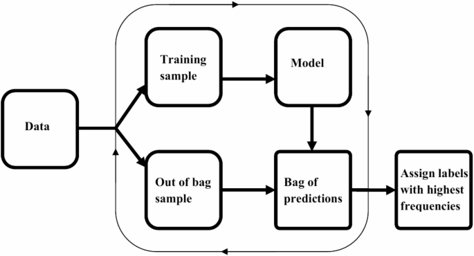
Overview of BamClassifier. A subsampling of equally sized samples is selected repeatedly without replacement. Each subsample is used to develop a median-supplement naive Bayes model and tested on the unused samples (out-of-bag samples). The predictions of the out-of-bag samples are aggregated into a consensus bag, bag of predictions, where labels for each unique instance is assigned the majority class or label among its predictions.

Sub-sampling for training and testing model

For a given data with n instances, a sub-sampling of approximately equally sized samples is randomly selected repeatedly without replacement from the original data. This sampling continues until every instance in the original set has been included in a subsample. For each subsample, a classifier is developed and tested with the out-of-bag samples. This sampling technique allows every instance to be included in developing models, and as well as testing the model at some point in the process. Here, we let B denote the number of sub-samples that are drawn from the original data made up of n instances. The predictions of the out-of-bag samples are aggregated into a consensus bag, referred to as bag of predictions. In the bag of predictions, the label for each instance is the majority class or label.

Building a bamclassifier

For every subsample, a median-supplement naive Bayes classifier²² was developed as the learning model. Here, it is incorporated in the models for assessing iron deficiency based on serum ferritin levels. The difference between instances of the ID positive and ID negative statuses is determined. Let this difference be m. With this determined, an m by k matrix of Latin Hypercube²⁷ with uniformly distributed probability values are generated for k features of the selected subsample. In this way, each column of the matrix will correspond to the features of the samples. A scalar multiplication of the median of each feature and corresponding column (vector) of the Latin Hypercube is determined. That is, suppose \(x{}_{i}\) represents the vector of i-th attribute values in a sample, and \(x_{i}^{\prime }\) is the corresponding column in the m by k matrix, the supplementary data corresponding to the i-th attribute, denoted by \(s_{i}\) will be given by Eq. (1):

where \({med\left( {x_{i} } \right)}\) is the median of the i-th attribute values in a sample. These supplementary observations corresponding to i-th attribute is included in the training set as additional sets of instances for attribute i. That is, if there were j observations for the attribute i in the training set, it will be extended to (j + m) observations such that the labels of the new instances will be the lesser label of the original instances. For example, suppose for attribute i, there are 10 samples with 4 ID positive and 6 ID negative statuses in training set. Then, the difference between the numbers of statuses, m, is 2 (6 minus 4), and two additional instances with the ID positive labels will be added to the 10 instances to make it 12. The values of the attributes for the two additional (supplementary) instances is given by scalar multiplication of the median of attribute i and the column vector corresponding to the i-th attribute of the m by k matrix.

Applying this to every column of the m by k matrix results in the transformation of the m by k matrix which becomes the supplementary data included in the subsample from which the classifier is inferred. This balances the differences between the ID statuses to equal numbers of instances to improve the accuracy of every model built from each subsample as the supplementary data will bear the label of the lesser ID status in the original subsample. Every model inferred from the subsamples by this approach improves its effectiveness in predicting the out-of-bag samples. The aggregation of all the predictions is stored in a bag of predictions where labels are assigned to every test instance based on the number of consensus predictions. For every instance, the label with the highest frequency among its predicted labels is assigned to it. The steps involved in building BamClassifier are outlined below:

1. 1.

   Specify the size of subsamples or folds for model building.

2. 2.

   Sample a subsample from the initial set without replacement.

3. 3.

   Build a median-supplement naive Bayes model on the selected sample.

4. 4.

   Predict the out-of-bag sample instances (i.e., predict every other instance).

5. 5.

   Repeat steps 2 to 4 until every instance has been included in exactly one sample for model building in step 3.

6. 6.

   Aggregate all predictions in step 4 into a consensus bag, called bag of predictions.

7. 7.

   For each instance, assign the most probable label, which is indicated by the label with the highest frequency.

Naive Bayes method

Using the Bayes theorem, it can be shown that for a given set of features, G, corresponding to several instances of ID statuses, the probability that any ID assessment is classified into a single ID status, say positive (\({C_{{ + ve}} }\)), is given by Eq. (2):

where \({P\left( {G|C_{{ + ve}} } \right)}\) is probability of instance G, given that the sample ID status is positive, \({P\left( {C_{{ + ve}} } \right)}\) is the probability that ID status is positive, and P(G) is the probability of observing the set of features G. In this way, the ID status of any sample is determined to be positive if this class has the highest posterior probability. However, it is assigned negative if the negative class has the highest posterior probability. This approach to classification assumes that distribution of the effective variables is independent, and this is consistent with the current measured attributes ID statuses’ data. This suggests that the conditional probability on the right-hand side of Eq. (2) can be expressed as Eq. (3) for any i-th feature of k features, \({g_{i} }\), under consideration in the ID assessment problem.

Performance measures

For benchmarking, the proposed method is compared to other well-established best performing probabilistic and tree-based methods namely naive Bayes, Bayesian networks, logistic regression, random trees and random forest methods implemented in Weka²⁸. These methods are compared on the basis of performance indicators which are true positive, true negative, false positive and false negative. When an instance of ID positive status is correctly predicted as positive, it is counted as true positive (TP). When an instance of ID positive status is wrongly predicted as negative, it is counted as false negative (FN). When an instance of ID negative status is correctly predicted as negative, it is counted as true negative (TN). When an instance of ID negative status is wrongly predicted as positive, it is counted as a false positive (FP). These observations are assessed in cross-validation used to evaluate every method in this study. While a 4-fold is used for evaluation of methods on actual datasets, a 10-fold cross-validation is used for the simulated datasets. The use of cross-validation reduces the likelihood of overfitting by the various methods used in this study.

With these indicators, the abilities for the methods are evaluated using the following measures:

The maximum value for the metrics accuracy, precision, specificity, and sensitivity is 100% and a good model approaches this maximum value as much as is possible. The accuracy measures the classification rates for each method in assessing ID status for any sample. While sensitivity measures the methods’ performances on predicting ID positive instances, specificity indicates the performance on correctly distinguishing instances that are not ID positive status. Precision assesses the predictive performances relative to the false positive counts. On the other hand, the diagnostic odds ratio (DOR), representing the ratio of the product of correct predictions to false predictions, is expected to be greater than one (1) for good models although it is also desirable to have large value.

In the overall assessments of how well a method performs, the trade-off between sensitivity and false positive rate (1 – specificity) are visualized in the receiver operating characteristics (ROC) curve^29,30. The area under the ROC curve (AUC) further provides an indication of how well a model performs indicating discriminating power in deciphering different ID statuses as has been shown in machine learning applications in the past^31,32. For any model, the AUC can reach a maximum of 100%. The higher the AUC, the better the model. Good models are expected to have a higher AUC compared to any random model. The proposed method and its analysis were implemented in the R statistical software version 4.2.2.

Statistical tests

Analysis of data to assess normality and to compare equality of means of ferritin levels between groups of samples were conducted in R. Shapiro test was used to verify normality of the data. The data was not found to be normally distributed (p < 0.001). Therefore, a Mann-Whitney test was used to compare differences between groups of samples. All statistical testing of significance was performed at 5% level of significance.

Assessing the stability of performance of BamClassifier

In order to assess stability of the model’s performance, 100 bootstrap samples were generated from the original dataset. The model was trained on each sample and tested on the corresponding out-of-bag (OOB) data. Performance metrics were recorded for each iteration, and the means, standard deviations, and 95% confidence intervals were calculated to assess the model’s stability. Additionally, a line plot was used to visualize performance metrics across the bootstrap iterations, illustrating the trends and consistency of the model’s performance over time.

Robust assessment of BamClassifier

We conducted robust assessment of the proposed method. In doing this, we assessed its performance by varying factors such as class imbalance, feature noise, and data distribution. The original datasets were not found to follow any known standard distribution. Therefore, an empirical distribution was assumed as an estimate of the underlying distribution of each attribute or feature²⁹. This enabled us to sample 1000 instances from each distribution. Imbalanced labels (90:10) were randomly assigned to the instances, and the model was evaluated to observe its performance on imbalanced data. In order to assess the effect of feature noise, we simultaneously introduced noise of varying levels into two features in two experiments, and half of the features in another experiment. Details are provided in the supplementary material with implementation code. In order to further vary data distributions, we sampled 1000 samples for each feature from a Gamma distribution with shape and rate parameters aligned with the original features to approximate the underlying characteristics. Details of these robust assessments are provided in the supplementary material with implementation code. For each robust assessment, a 10-fold cross-validation was performed on datasets of 1000 samples.

Code availability

All computer codes supporting this study are available as supplementary material.