Application of deep learning for fruit defect recognition in Psidium guajava L

Table 1 presents the training results. In the overall image database, a total of 1701 images were marked using thirteen labels (as shown in Table 2). A total of 4044 labels were applied, and the overall false negative rate and false positive rate were 5.03% and 6.62%, respectively.

Deep learning

During training, assessments were made using box loss, object loss, and class loss, with values closer to 0 indicating higher accuracy. We randomly retrieved 70% of the images in the database as training data (1190 images), and the remaining 30% served as test data (511 images). The appearance defects were divided into 13 classes, as shown in Table 2. We utilized the Yolo v4-coco pretrained network architecture and added the above database to retrain the network weights. It was executed on a computing host with an i7 processor with a processing speed of 2.1 GHz, 64G RAM, and an RTX 3080 graphics card. The training took a total of two days, two hours, and 47 min. With the training set, the total loss, box loss, object loss, and class loss were 0.2576, 0.19043, 0.026229, and 0.040938, respectively.

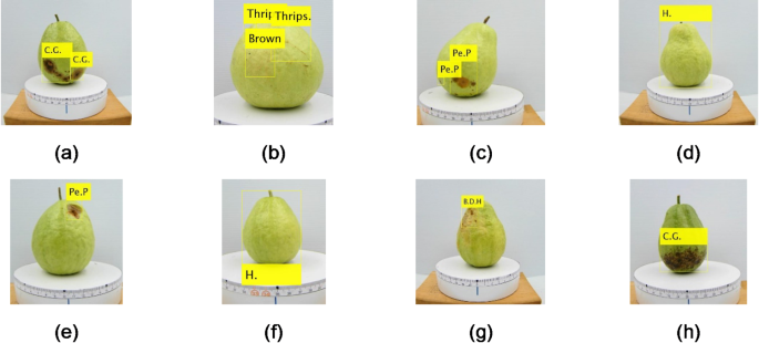
Figure 1 exhibits some of the image recognition results of the training and test sets. Figure 1(a) ~ 1(d) present some of the image recognition results of the training set. Figure 1(a) shows an example of Colletotrichum gloeosporoides in the training set. As shown in Fig. 1(b), a single image may contain more than one type of defect; this figure shows damage from thrips and browning. Figure 1(c) shows an example of Pestalotiopsis psidii and Fig. 1(d) displays a healthy fruit with no defects. Figure 1(e) ~ 1(h) present some of the image recognition results of the test set. Figure 1(a) shows an example of Pestalotiopsis psidii in the test set. Figure 1(f) displays a healthy fruit with no defects. Figure 1(g) shows an example of damage from Bactrocera dorsalis Hendel. Figure 1(h) shows an example of Colletotrichum gloeosporoides.

Experiment results: (a)~(d) training images; (e)~(h) test images.

The term false positive (FP) refers to non-defective cases that are misidentified as defects. They are identified by comparing the results of automatic detection using the trained network with manually-marked samples using the formula in Eq. 1. The term false negative (FN) refers to defective cases that are missed in the detection process. They are determined using Eq. 2. True positives (TP) are calculated as the total number of samples minus the number of missed detections. Table 1 exhibits the training and test set data for each class. In the random training set, the false negative rates in each class were less than 1%, and the false positive rates were less than 13%. The two classes with the highest false positive rates were Planococcus minor (P.M.=13%) and damage from thrips (Thrips = 11%). In the manually-marked samples, the false negative rate was 0.17% and the false positive rate was 5.33%.

To prevent overtraining, which would increase the number of accurately recognized results in the training set but lead to abnormal situations with images not in the training set, we used the remaining images as the test set and employed the training set with manually-marked samples to test whether overfitting existed in the trained network weight. In the test set, the class with the highest false negative rate was manmade damage (M.D.), which had a false negative rate of 38%. This was followed by 32% in the physical damage from branches (P.D.) class (both classes had few samples in the database, and there were wide variations between samples). These were followed by damage from Lepidoptera larvae (Le.=29%) and damage from Bactrocera dorsalis Hendel (B.D.H = 29%). The average false negative rate was 16%. The false positive rates of each class were less than 36%. The two classes with the highest false positive rates were browning (Brown = 36%) and physical damage from branches (P.D.=30%). In the manually-marked samples of the test set, the false negative rate was 15.82% and the false positive rate was 11.29%.

The total number of the training and test sets was 4404. Colletotrichum gloeosporoides had the highest number with 1120; the total number of false negatives of Colletotrichum gloeosporoides in the training and test sets was 27, and the false negative rate was 2.35%. The total number of false positives in the training and test sets was 62, and the false positive rate was 5.25%. There were 6 instances of sunburn, with 1 false negative for a false negative rate of 14.29%. There were 20 instances of manmade damage (M.D), with 5 false negatives for a false negative rate of 20%. There were 110 instances of Planococcus minor (P.M.), with 19 false positives for a false positive rate of 14.73%. There were 129 instances of physical damage from branches (P.D.), with 27 false positives for a false positive rate of 17.31%. Overall, the false negative rate was 5.03% and the false positive rate was 6.62%.

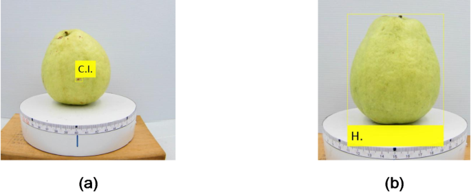
Recognition results: (a) smallest recognition result: 13 × 14 pixels; (b) largest recognition result: 266 × 312 pixels.

In the experiment results, the smallest and largest objects detected were a chilling injury of 13 × 14 pixels and a healthy fruit of 266 × 312 pixels, respectively, as shown in Fig. 2.

Further analysis was conducted to assess the robustness of the model against FNs and FPs. This was achieved by determining the number of TPs, FPs, and FNs in the training and test datasets, as summarized in Table 1. The initial analysis revealed no FPs or FNs in the training set, indicating that the training results were based on reliable data.

To further assess model performance²¹, 200 images without the object of interest were added to the test dataset. The model was then assessed in terms of accuracy, precision, recall, and F1-score. Accuracy was defined as the proportion of correct predictions across the entire sample. Precision was defined as the proportion of samples identified as positive that are actually positive (TPs), while recall was defined as the proportion of actual positive samples that were correctly identified by the model. The F1-score indicates the harmonic mean of precision and recall, providing a single measure that balances both aspects.

The data in Table 1 was subsequently used to compare the predictions versus the ground truth based on the numbers of TPs, FPs, FNs in the training and test sets, irrespective of specific categories. An additional 200 images without the object of interest were added to the test dataset. These images were correctly classified in the group without objects from any category, resulting in 200 TNs (see Table 3).

Table 4 Lists the accuracy, precision, recall, and F1-scores calculated based on the values ​​in table 3. All values for the training set exceeded 94.5%, indicating good model stability. The values for the test set exceeded 75%, which is considered satisfactory. The overall mean value across datasets was above 88%. Taken together, these results highlight the model’s robustness and stability without evidence of overfitting.

This study performed real-time detection using a pretrained YOLO v4-COCO object detection model running on a system with an Intel i7 2.1 GHz processor and an RTX 4090 graphics card. The resolution of each image in the stacked test dataset was 3840 × 2160 pixels; however, none of the detected objects exceeded 266 × 312 pixels in size (i.e., approximately one-tenth of the image resolution), as shown in Fig. 2(a). Setting the region of interest (ROI) to 1000 × 1000 improved the detection speed to 12 FPS. When applied to the image dataset, the system achieved a false negative rate (FN) of 5.03%, a false positive rate (FP) of 6.62%, and accuracy of 88.15%.