A robust machine learning approach to predicting remission and stratifying risk in rheumatoid arthritis patients treated with bDMARDs

Patient demographics and baseline characteristics

In this study, we initially included 4344 patients from the Bioreg dataset. After applying inclusion criteria and removing patients who had not had any follow-up visits, 1,494 patients remained. Next, we excluded patients who did not have the DAS28-ESR Score recorded at the six-month follow-up. This resulted in removing 271 patients, leaving a final cohort of 1,223 patients. Further data cleaning was performed to remove visits that were not necessary for the predictive modeling (see “Data preprocessing” section). After this process, patients were labeled based on their remission status at six months according to the DAS28-ESR score. Table 1 presents the baseline characteristics of the 1,223 patients, including the mean and standard deviation (SD) or percentage of key clinical features. The table also compares baseline characteristics between patients who achieved remission and those who did not at six months. Of the 183 RA patients screened at Erlangen, 154 had at least one follow-up visit six months from baseline. The remaining 29 patients were excluded for not meeting this criterion. Table 2 summarizes the baseline clinical characteristics of the 154 RA patients, stratified by their six-month response.

Predictive models

Classification performance before calibration

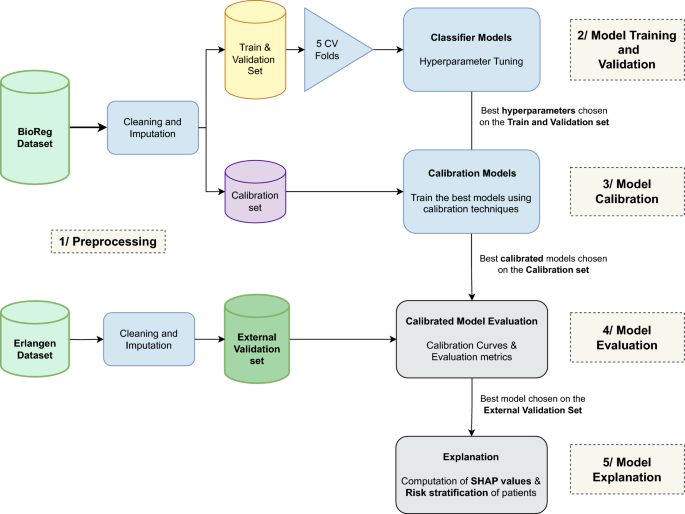
The predictive models AdaBoost, Random Forest, Support Vector Machine (SVM), and XGBoost, were trained and evaluated on the Bioreg dataset. After hyperparameter tuning, their performance was assessed on an external test dataset (Erlangen), representing an independent patient population. The evaluation metrics, summarized in Table 3, reflect the ability of each model to predict remission after 6 months and generalize to unseen data.

Among the models, AdaBoost demonstrated the most consistent performance across the majority of metrics, showcasing its ability to strike a balance between sensitivity (recall) and precision. XGBoost, on the other hand, achieved the highest AUC-ROC, indicating superior discrimination capability in distinguishing between remission and non-remission cases. Despite this, AdaBoost emerged as the most balanced model overall, particularly for predicting remission after six months, due to its strong performance across multiple metrics and its ability to generalize effectively to the external test dataset. The results highlight the strengths of ensemble methods like AdaBoost and XGBoost, which combine predictions from multiple learners to improve accuracy and robustness. Ensemble models are generally more resilient to overfitting and better equipped to handle the variability inherent in external datasets, as demonstrated by their performance on the Erlangen dataset.

For a visual comparison of the models’ performance, refer to Supplementary Fig. 1.

Model calibration and performance

We evaluated the calibration performance of four models to assess the reliability of their probability estimates in predicting remission. The calibration curves assess the alignment between the predicted probabilities and the observed outcomes. We applied various calibration methods to refine these estimates, including Platt scaling (sigmoid), Isotonic regression, Spline calibration, and Beta calibration. Figures 2, 3, 4, and 5 show the calibration curves for each model before and after calibration. Model performances were evaluated using Brier score, Accuracy, Precision, Recall, F1-Score, and Matthews Correlation Coefficient (MCC). Tables 4, 5, 6, and 7 summarize the results before and after calibration.

AdaBoost calibration performance

The calibration curves for the AdaBoost model (Fig. 2) illustrate the impact of calibration techniques on the reliability of the predicted probabilities. The diagonal line, shown as a gray reference in the calibration plot, represents perfect calibration, where the predicted probabilities align exactly with the observed outcomes. In other words, a predicted probability of 0.7 would correspond to an actual event rate of 0.7, and so on. Before calibration, the predicted probabilities of the uncalibrated AdaBoost model showed deviations from the ideal diagonal line, suggesting some degree of over- and underestimation in the predictions. This is further supported by the higher pre-calibration Brier score of 0.20, indicating room for improvement in the predicted probabilities.

After applying calibration techniques, isotonic regression achieved the best overall calibration performance for the calibrated AdaBoost model, reducing the Brier score to 0.13 and closely aligning the predicted probabilities with the observed outcomes. Spline and beta calibrations also improved, with Brier scores of 0.14, while maintaining high classification performance metrics.

The summary of performance metrics for both the uncalibrated AdaBoost model and the calibrated AdaBoost models is presented in Table 4.

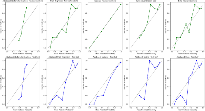
Calibration curves for AdaBoost across different calibration techniques (Platt, Isotonic, Spline, and Beta) for the calibration and test datasets. The isotonic calibration method provided the best alignment between predicted and observed probabilities, on both the calibration set and the test set.

SVM calibration performance

The calibration curves for the SVM model (Fig. 3) show deviations from the ideal diagonal line in the uncalibrated model, particularly in the lower- and middle-range of the predicted probabilities. This indicates that the uncalibrated SVM model overestimated probabilities, assigning higher likelihoods to positive outcomes than warranted. The pre-calibration Brier score of 0.17 further highlights the need for refinement in probability estimation.

After calibration, Beta and Spline methods offered slight improvements, particularly in aligning predicted probabilities with observed outcomes in the mid-range probabilities. However, the calibrated SVM models still exhibited miscalibration at the extremes of the probability distribution, and the Brier score marginally increased to 0.18 after Beta calibration, suggesting limited success in improving overall probability estimates.

From a classification perspective, minor improvements were observed following calibration. The F1-Score increased from 0.77 to 0.78, and the Matthews Correlation Coefficient (MCC) improved from 0.52 to 0.54, indicating slightly better agreement between predictions and actual outcomes. Recall rose modestly from 0.82 to 0.84, while precision remained stable. These changes suggest that calibration had a limited but measurable impact on the model’s ability to classify remission outcomes correctly.

While calibration techniques brought some predicted probabilities closer to the ideal diagonal line, particularly in mid-range probabilities, they did not resolve miscalibration at the extremes. The results suggest that the calibrated SVM models, while showing modest improvements in classification metrics, cannot be reliably used for clinical applications. The performance metrics for the SVM model before and after calibration are summarized in Table 5.

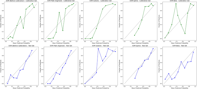
Calibration curves for SVM before and after different calibration techniques (Platt, Isotonic, Spline, and Beta) for the calibration and test availsets.

Random forest calibration performance

The Random Forest model exhibited a relatively well-calibrated pre-calibration curve compared to other models (Fig. 4). The pre-calibration curve shows that the predicted probabilities were already reasonably well-aligned with the actual outcomes, as indicated by a Brier score of 0.157 and a high classification accuracy of 84.42%. Additionally, the model achieved an F1-Score of 0.842 and a Matthews Correlation Coefficient (MCC) of 0.689, reflecting strong classification performance before calibration.

Various calibration methods yielded mixed results. Spline calibration produced the best calibration results, with the post-calibration curves demonstrating better alignment with the diagonal, particularly in the middle probability range. However, Beta calibration worsened the probability estimates, leading to an increase in the Brier score to 0.226. This increase in the Brier score indicates that Beta calibration did not improve the calibration quality.

Despite the increase in the Brier score, recall improved from 0.831 to 0.909 with Beta calibration, showing better sensitivity in identifying true positives. However, this came at the expense of accuracy, which dropped to 75.32%, and the F1-Score also declined to 0.787. After calibration, the MCC dropped to 0.533, suggesting a less balanced overall classification performance.

In contrast, Spline calibration resulted in more consistent performance, with the post-calibration curve closely aligning with the diagonal. While the overall classification performance did not significantly improve, the calibrated probabilities showed better accuracy across a broader range of predicted probabilities, especially in the middle ranges, without introducing significant degradation to the Brier score.

In summary, Spline calibration provided better alignment with the diagonal line and more stable performance, while Beta calibration led to a deterioration in calibration quality. Therefore, Spline calibration can be considered the more effective method for improving the calibration of the Random Forest model.

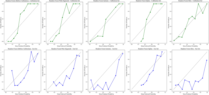
Calibration curves for Random Forest before and after different calibration techniques (Platt, Isotonic, Spline, and Beta) for the calibration and test availsets.

XGBoost calibration performance

Figure 5 presents the calibration curves for XGBoost on both internal and external validation availablesets. Without calibration, the probability estimates could be unreliable. The model overestimated probabilities in the lower ranges and underestimated them in the higher ranges, as indicated by a Brier score of 0.179. Despite this, the uncalibrated model performed well, achieving an accuracy of 83.77%, an F1 score of 0.834, and a Matthews Correlation Coefficient (MCC) of 0.676.

Substantial improvements in probability estimates were observed after calibration, particularly with beta calibration. Beta calibration reduced the Brier score from 0.179 to 0.152. Furthermore, while the accuracy decreased slightly to 80.52%, the recall increased from 0.818 to 0.883, indicating a better ability to identify true positives. The F1 score remained relatively high at 0.819, and the MCC was 0.618 after calibration. The AUC-ROC score remained stable at 0.889, demonstrating consistent discriminative ability before and after calibration.

Overall, Beta calibration provided the best calibration performance for the XGBoost model, leading to more accurate probability estimates, as reflected by the lower Brier score. While there was a slight trade-off in accuracy, the improvements in recall and calibrated probability estimates make Beta calibration the preferred method for XGBoost.

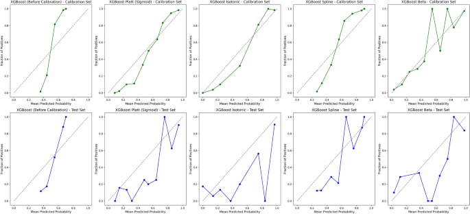
Calibration curves for XGBoost before and after calibration.

Best model for remission prediction and probability estimates

AdaBoost provided the best performance for remission classification and probability accuracy among all models tested without calibration. It achieved the highest accuracy (86.36%), F1-Score (0.86), and MCC (0.73), demonstrating strong classification capabilities. Additionally, its Brier Score of 0.134 indicated that it produced the most accurate probability estimates, outperforming the other models.

Calibration methods such as Spline and Beta improved the probability estimates of models like Random Forest and XGBoost, but they did not surpass AdaBoost’s performance.

In summary, AdaBoost with isotonic regression was the most effective model overall, making it the best choice for both accurate remission classification and reliable probability estimates.

Explainability and feature importance

To enhance interpretability and clinical utility, SHapley Additive exPlanations (SHAP) were applied to the test availableset of the AdaBoost classifier to quantify the contribution of individual features to the model’s predictions. The SHAP summary plot in Fig. 6 illustrates the top baseline features that had the most significant influence on the model’s prediction of remission.

The plot shows that the DAS28 Score at the baseline was the most influential feature, indicating its strong predictive power for remission outcomes. Other important features include the VAS score (based on patient assessment), age, and SJC, which were critical in shaping the model’s predictions. The SHAP values highlight the relationship between feature values and their impact on the model. Higher values of features such as DAS28 and age shifted the predictions towards non-remission. In comparison, lower values of these features were associated with a higher likelihood of remission. This explainability offers valuable insights for clinicians by identifying the key factors contributing to remission prediction and clarifying their directional impact on outcomes, enabling more personalized and informed treatment decisions based on these critical clinical indicators.

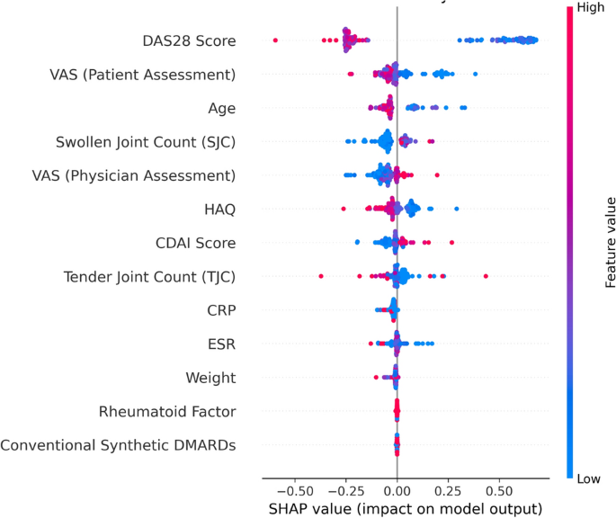
SHAP summary plot on the test availableset (Erlangen availableset) highlighting feature importance and directional impact on remission prediction. This plot illustrates the impact of baseline features on the model’s output for predicting six-month remission in rheumatoid arthritis patients before initiating bDMARD therapy. Each dot represents a patient, with the color indicating the baseline feature value (red for high, blue for low). Features like DAS28 Score, VAS (Patient Assessment), and Age have the highest influence, where higher DAS28 and VAS values at baseline reduce the likelihood of remission, while lower values increase it. This explainability supports clinicians in understanding how baseline clinical indicators influence predictions and informs personalized treatment decisions.

Risk stratification outcomes

The AdaBoost model demonstrated strong performance in estimating remission probabilities, with isotonic regression identified as the optimal calibration method. This was supported by a lower Brier score (0.13) and superior alignment between predicted and observed probabilities in calibration curves (Fig. 2).

Following calibration, patients were stratified into three risk categories based on their predicted remission probabilities: low risk (>0.66), medium risk (0.33–0.66), and high risk (<0.33). These thresholds were chosen to reflect clinically meaningful separation in treatment response probabilities. Figure 7 illustrates the distribution of remission probabilities within each risk group in the test set.

Baseline characteristics of patients differed substantially across the risk groups (Table 8). Patients classified as high risk presented with more severe disease activity at baseline, including higher DAS28 and CDAI scores, elevated inflammatory markers (ESR and CRP), and greater joint involvement. In contrast, patients in the low-risk group exhibited milder clinical profiles.

Observed remission outcomes reflected the predicted risk levels (Table 9). The remission rate was 89.7% in the low-risk group, compared to 24.1% and 15.8% in the medium- and high-risk groups, respectively. This clear gradient in treatment response validates the model’s ability to stratify patients into clinically meaningful categories and supports its utility for precision medicine in RA.

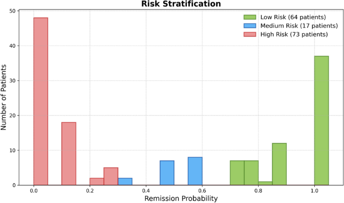
Risk stratification using the AdaBoost model calibrated with isotonic regression. Patients were categorized into low-risk (green), medium-risk (blue), and high-risk (red) groups based on their calibrated remission probabilities.