A feature explainability-based deep learning technique for diabetic foot ulcer identification

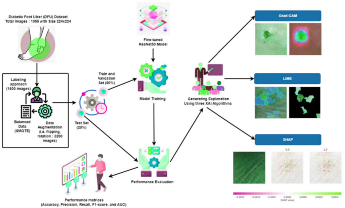
This study employs a model that has been previously trained to extract visual data from diabetic foot photos and uses DL to distinguish between healthy skin and ulcers. CNN, the algorithm uses heat maps or segmentation of regions to forecast ulcers. The DFU_XAI classification system is shown in Fig. 1. It incorporates three XAI approaches, six fine-tuned deep CNN models for model training, data augmentation, and performance measures. XAI-based transparent approach aids in finding biases and reducing AI model biases. A lack of feature explainability, an imbalanced dataset, and a poor supply of DFU datasets are some of the challenges. Here are several solutions: an augmentation method, a dataset balancer using SMOTE, and a visual attribute explanation using a combination of XAI and ResNet50 algorithms. Using the SNN technique, compare two photos of the same foot, and then use contrastive loss to identify which two images are similar and which are different. To improve the model’s ability to make decisions and enhance confidence and interpretability in clinical situations, explainability methodologies like ResNet, Grad-CAM technology, and SHAP values are included.

In contrast to LIME, which finds perturbation, SHAP employs a gradient explanation. Grad-CAM generates scores using gradients. Disparities in feature description, imbalance in the dataset, and lack of access to the DFU dataset were the three main problems in implementing the DFU_XAI framework. To address these concerns, add more data, use SMOTE to even out the dataset, and combine ResNet50 with three XAI algorithms—one of which is SNN—to make visual features more understandable. The experimental design process and outcome computation is shown in the DFU_XAI framework displays the sequential categorisation in Algorithm 1.

The sequential categorisation process of Algorithm 1 in the DFU_XAI framework explainability techniques like SHAP, LIME, and Grad-CAM within the framework. Describe how these tools enhance the interpretability of model predictions and contribute to clinical decision-making.

Explainability techniques SHAP, LIME, and Grad-CAM

SHAP (Shapley Additive Explanations)

• Objective: Quantifies the contribution of each input feature to model predictions, providing local explanations.

• Clinical Impact: Helps clinicians validate predictions by indicating which regions of the image are influencing the classification. Positive/negative contributions help align model predictions with clinical expectations and build trust.

LIME (Locally Interpretable Model-Agnostic Explanations)

• Objective: Breaks the image into superpixels, then perturbs them to see their effect on predictions.

• Clinical Impact: Highlights relevant regions (such as ulcer sites) that are useful for verification by clinicians. This helps identify biases or errors and increases clinicians’ confidence in the model.

Grad-CAM (Gradient-weighted Class Activation Mapping)

Purpose: Generates heatmaps that indicate which areas of the image are critical for the model’s prediction, by backpropagating gradients.

Clinical impact: Provides intuitive visualizations that indicate where the model is focusing. This aids in accurate ulcer localization, which is useful for diagnosis and treatment planning.

Objective of the paper

The main objective of this paper is to use deep learning models integrated with explainable AI (XAI) techniques to improve the diagnosis and localization of diabetic foot ulcers (DFUs). By incorporating XAI methods such as Grad-CAM, SHAP, and LIME, this framework brings transparency to the decision-making process of the model, allowing clinicians to understand and trust the predictions.

In addition, the use of data augmentation significantly improves model performance, which overcomes the challenges of limited and imbalanced datasets. Techniques such as rotation, scaling, and flipping reduce overfitting by increasing the diversity of training samples and improve the generalization ability of the model.

The combination of these state-of-the-art deep learning architectures, explainability tools, and data augmentation creates a robust, accurate, and interpretable system for DFU detection that helps clinicians make informed and reliable decisions.

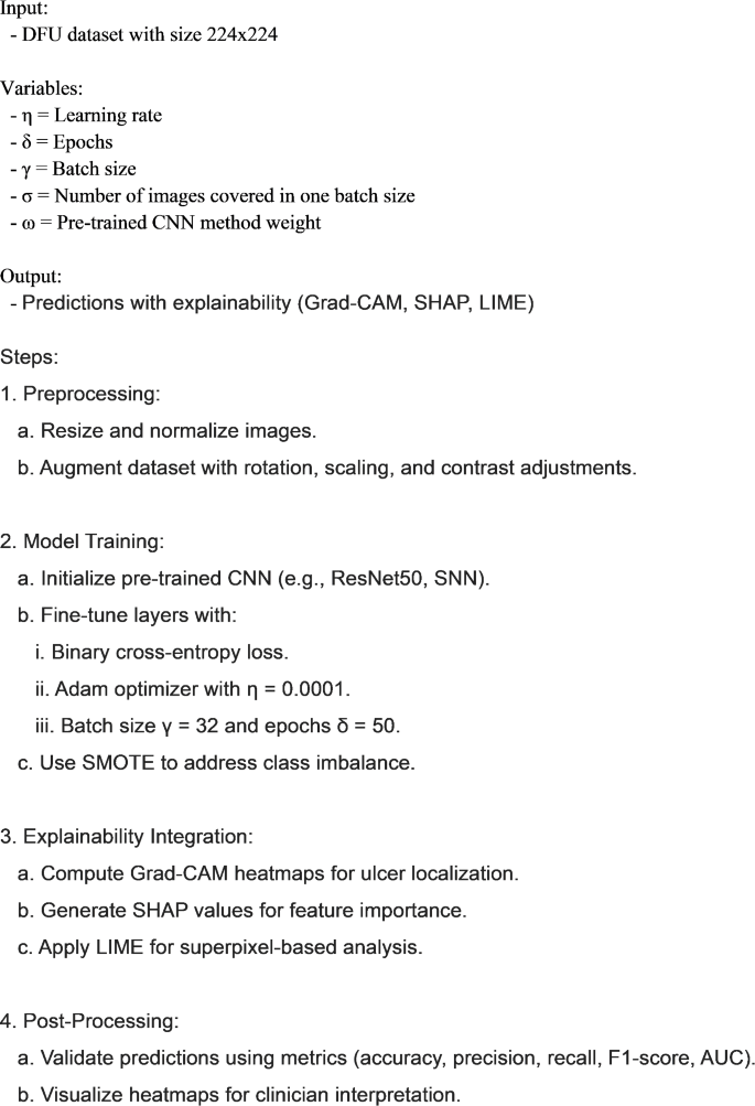
Planned DFX_XAI Outline for DFU Finding

Loss function: For the SNN, the contrastive loss function can be defined as.

Where: y is the label (1 for dissimilar, 0 for similar), D is the Euclidean distance between embeddings, m is the margin for dissimilar pairs.

The description of used dataset in this methodology as follows:

The diabetic foot ulcer dataset

To evaluate the model, data was gathered from 1050 skin patches that were donated by patients. Only 540 of the patches were determined to be normal, suggesting healthy skin; 510 were determined to be aberrant and classified as ulcers. On the other hand, a large amount of labelled data is necessary for the proper operation of a DL method. It could take a lot of time and money to gather a lot of medical data. Therefore, DL models may be improved and overfitting reduced by using image labelling, data enhancement, transfer learning, and regularisation. A solution to this problem is the use of patch labelling to enhance the size of the dataset. It sorts data by selecting the most important parts of a big sample and assigning them to the appropriate category. The first research used a 224-pixel-high by 224-pixel-wide sliding window to recover the Region of Interest (ROI) from each sample. The window was moved from top left to bottom right. According to the areas of normal and ulcer skin, patches are categorised as either healthy or ulcer. In contrast, the DFU_ XAI architecture enhanced the efficiency of DL models by concentrating on individual DL traits rather than the whole sample. The parts associated with ulcers were marked in larger samples. Important DL information is extracted for classification using this method. When training a DL model, using appropriate DL data helps to prevent overfitting by reducing memory allocations and compute demands. This method yielded 1680 image patches, 830 of which were normal and 850 of which were ulcer related. Picture examples that have been cropped are shown in Fig. 2.

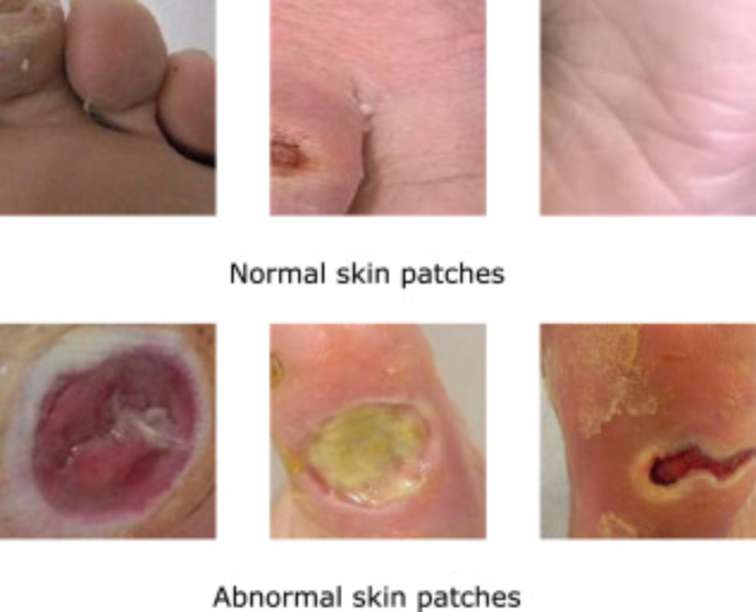
Ulcer Skin normal and abnormal Images [Available at: google.com/search/images].

By employing new colour spaces to enhance contrast, resizing, relocating, and randomly scaling data, expand both its size and diversity. In this study, 1680 skin patches were rotated at angles of 90° and 180°. Following this process, the DFU data set was created by the researchers. It contains 3100 skin patches, out of which 1710 photographs depict aberrant ulcers, and 1490 pictures show healthy, usual skin. The DFU dataset is divided into two sets, one for training and one for testing, via the “train_test_split” algorithm. 10% of the information from the training set is re-split using the same procedure for validation. The dataset for this investigation is summarised in Table 2. Using SMOTE, this approach tackles imbalanced DFU datasets. Overfitting caused by random oversampling is, however, addressed by this strategy. Due to imbalances in the datasets, DL models might be biased. SMOTE distributes data evenly to reduce bias. Model performance is impacted by efforts to minimise bias and collect minority label characteristics. The results of models may not always be improved by SMOTE. It can generate synthetic samples that aren’t always realistic. The distribution of minority labels may not be correctly reflected by these hypothetical samples. When samples from the majority and the minority overlap, this can cause information from the dominant label to seep out.

1. 1.

   Dataset Composition and Size

2. 2.

   Preprocessing Techniques

   • Patch Labeling:

   • Sliding Window Approach:

3. 3.

   Data Augmentation

4. 4.

   Addressing Dataset Imbalance

5. 5.

   Train-Test Split

6. 6.

   Significance of Preprocessing and Augmentation

Reducing computational demands by focusing on key image features.

Strong hardware and time are required for a CNN model with many training parameters. These concerns may be resolved by transferring variables and weights from existing dataset techniques to the new model. Levels may be bridged and more levels added using Transfer Learning and transferred parts. This method is less computationally demanding and faster even with little datasets. Data is expensive, time-consuming, and difficult to get by, yet traditional AI must train its model. This issue is addressed, DFU_XAI used ImageNet weights derived via transfer learning. First, the DFU_XAI framework’s training time is reduced using this method. Second, it improves the success rate of the framework. Third, it allows for the insertion of more data and the adjustment of parameters during model training, which improves the framework.

This research uses six state-of-the-art CNN methods for classification: ResNet50, DenseNet121, InceptionV3, MobileNetV2, Xception, and SNN. Architecture, classification accuracy, and explainable prediction were the deciding factors in the selection of these cutting-edge models. Structures and modules differ from model to model. The following networks provide outputs from their siamese layers: Xception, ResNet, DenseNet, InceptionV3, MobileNetV2, and InceptionV3 inverted. Xception makes use of depthwise separable convolution blocks. When it comes to ImageNet, these networks shine. The input image’s DL data was obtained using pre-trained weights to improve the model’s performance. Big datasets are no match for these models. These CNN models used transfer learning with pre-set weights. By exchanging data and weights, models may train more quickly and efficiently. Performance is improved by combining pre-trained models with fine-tuned layers. The data and split ratio were used to train and evaluate six pre-trained models. These models have six fine-tuning layers to enhance performance. Layers that altered the model’s pre-trained weights enhanced DFU_XAI. Refinement layers categorise DL characteristics that have been retrieved. The optimised layers enhanced the model’s functionality.

Residual network

Robust architecture for DL Residual Network (ResNet), short for Residual Network, which is has shown promise in many picture classification tasks, one of which is the detection of DFUs. ResNet is a DL system that uses residual learning to address the vanishing gradient problem and capture intricate patterns in medical images. ResNet learns complex features from high-resolution images, allowing it to reliably distinguish ulcerous from non-ulcerous regions in DFU identification. The use of ResNet in conjunction with explainability techniques such as Grad-CAM and salience maps allows for the visualisation of the method’s procedure for making decisions. With the help of this partnership, healthcare professionals are better able to accept and evaluate the model’s indications, which in turn improves their ability to make impartial decisions²⁰.

Convolutional neural networks

Tasks requiring object recognition, such as image segmentation, detection, and classification,

are well-suited to DL techniques like CNNs, often called “ConvNet”. One kind of DL that can find patterns in program and image data is CNNs. Spiral algorithms exploit a data leak to trick the recommendation system into giving an inaccurate result by pushing the recommendation system over the data.

A feature map depicting the input data’s structure as a function of features is the end product. Using the principle that nearby pixels have stronger correlations than distant ones, CNN implements²⁴. In this case, Fig. 3 shows the pooling process that the Max Pooling layer employs, which involves sliding a two-dimensional filter over each feature map channel. The feature maps are reduced in size by the pooling layer, which condenses all features within the coverage region of the filter. As a result, the network does not have to learn as many parameters, and its burden is mitigated. There are several types of pooling layers, including max, average, and global.

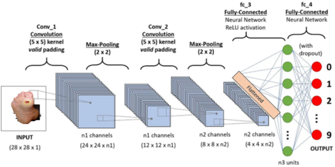
Framework for number recognition with CNN’s.

DL Method is used for the detection of DFUs; CNNs and similar models excel at processing images. CNNs can identify the intricate patterns and textures seen in DFUs because, via convolutional processes, they dynamically learn the spatial arrangement of features from input photos. By stacking several convolutional layers, CNNs accurately identify DFUs by capturing edges, textures, shapes, and lesions. To find the parts of the foot picture that have the most impact on the model’s predictions, CNNs combined with explainability techniques like Grad-CAM technology and saliency maps like DFU_XAI may be employed. By exposing the model’s decision-making process, increases diagnostic accuracy, empowers clinicians to trust AI-driven judgements, and ultimately leads to better patient outcomes. A strategy called XAI is used to incorporate the most significant elements of the trained method. This article describes in detail the three most used XAI methods for visual analysis: Grad-CAM, SHAP, and LIME.

Locally interpretable explanations and model-independent

The goal of the LIME method is to provide detailed justification for each calculation made by a black box method. A key idea behind LIME is to simplify and make more transparent a “glass box” model to approximatively simulate the local behaviour of a “black box” model. This will make interpretation much easier. By activating or deactivating super pixels selectively, LIME distorts visuals. This technique determines the significance of continuous super pixels in the output class’s original image and then disseminates that information. To make ML systems more trustworthy, LIME shows how the input features of CNN models affect predictions, which increases model interpretability and transparency. To use LIME, the first step is to divide an image into super pixels²⁵. The count of super pixels determines the region’s segmentation. Hyper pixels are adjacent pixels that share the same hue and position. This method produces more thorough and precise segmentation, which aids in locating zones that may forecast the output class. LIME approximates the black box model with an easier interpretable model to explain model predictions locally. Super pixel activation and deactivation perturb images, revealing model decision-making areas.

Weighted gradient activation mapping for classes

In typical CNN models several blocks are combined for feature extraction and categorization. A fully connected layer in the Classification block calculates probability scores from the SoftMax layer using the recorded features. In the end, the classification results of the model are generated with the likelihood score, which has the most value. By selecting the category that most closely matches the input image, the accuracy and performance of the model can be improved. Without modifying the network architecture or training, Grad-CAM provides visual explanations. This technique finds important areas of the image and uses the gradient of the feature map of the final convolutional layer to highlight the components that have the greatest impact on predicting the outcome. Grad-CAM pinpoints important areas of a picture to make the model more transparent and easier to comprehend, which in turn makes the model’s forecast clearer to the user. Huge gradients impact the accuracy of Grad-CAM picture predictions. Visualisation methods such as Grad-CAM and GradCAM + + assess a convolutional layer of a CNN by extracting quantitative and qualitative information about the layer’s inner workings via the identification of distinct image characteristics. You can fix Grad-CAM’s low heatmap resolution with Grad-CAM++. Based on the results, Grad-CAM and GradCAM + + have the potential to improve the network’s ulcer analytics capabilities by accurately locating the ulcer images. Grad-CAM produces pictorial clarifications by drawing attention to crucial regions of a picture that impact the model’s forecast. By providing higher heatmap resolution, Grad-CAM + + enhances Grad-CAM and makes it easier to localise ulcers in photos¹⁸.

Shapley additive explanations

Specifically, the SHAP method offers local explainability for text, picture, and tabular datasets. Subtractive feature importance is determined by averaging the feature space’s marginal contributions. SHAP values illustrate the impact of every input attribute on the model’s anticipated output. To improve the interpretability and transparency of decision-making in DL models, the DFU_XAI outline employs XAI methods such as GradCAM, SHAP, and LIME. The superpixel is retrieved from the expected samples using LIME in this method. The DL model’s transparency is enhanced by the acquired pixels. SHAP may provide both positive and negative numbers to describe the judgements made by DL models in different samples. These features make DL models more interpretable and transparent in their decision-making process¹⁸. To create the heatmap, Grad-CAM employs the last convolution layer of the DL model. The methods judgement is then made clear by highlighting these heat maps. The decision-making process may be fully understood by looking at the SHAP values, which show how each feature contributed to the model’s output. This method explains how each input characteristic affects the predictions by producing positive and negative values.

Siamese neural network

Two comparable networks that examine syntactic networks between different classes make up the SNN, a sign verification technique. They work side by side to create header graphics and divide up the weights. Knowledge regarding parallel processing, useful for classification or similarity measure, may be acquired using this CNN architecture. Improved heading representations are a result of the Siamese effect on animate nerve organ networks’ evaluation of heading correspondences. To make positive pairings more similar and negative pairings less similar, that are employed contrastive loss, penalises dissimilar samples if they are too near to the given margin. Medical image analysis makes use of SNNs to compare and develop functions of similarity between input items. Achieving symmetric learning is made possible by these networks’ identical subnetworks, which share parameters and weights³⁵. They find the distance metric between embeddings and use it to create a fixed-size vector that represents the higher-dimensional representation of the input picture. Improved classification efficiency, extensive feature learning, and ulcer development/healing tracking are all possible using SNNs. They may be added to other deep-learning models to boost accuracy, used to evaluate the network’s performance in classification and matching, and tested on a separate dataset. The structure of an SNN is shown in Fig. 4.

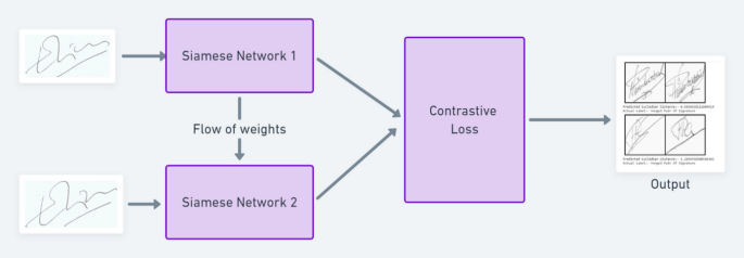
The categorisation and analysis of DFU is facilitated by the use of SNN’s, which exhibit strong performance in similarity identification and feature learning. By incorporating them into DFU processes, diagnostic accuracy and patient outcomes are enhanced.

Comparative Performance comparative performance of the six deep learning models.

The DFU_XAI framework integrates six advanced deep learning models—Xception, DenseNet121, ResNet50, InceptionV3, MobileNetV2, and Siamese Neural Network (SNN)—to improve the diagnostic accuracy and explainability of diabetic foot ulcers (DFUs). Each model offers a distinct strength with its unique architectural features.

Xception uses depthwise separable convolutions, which significantly reduces parameters and increases computational efficiency. It is suitable for large datasets but is weak in capturing complex DFU feature interactions.

DenseNet121 uses dense connectivity, in which every layer is connected to all previous layers. It improves gradient flow and helps to robustly extract intricate DFU features.

ResNet50 introduces residual connections that solve the vanishing gradient problem. It helps to train deeper networks and can accurately distinguish high-resolution medical images.

InceptionV3 uses multiple filter sizes that capture multi-scale features. It is effective in detecting DFU characteristics at different resolutions but requires more computational resources.

MobileNetV2 is an efficiency-focused model that uses inverted residuals and linear bottlenecks. It achieves moderate diagnostic accuracy and performs best in resource-constrained environments such as mobile diagnostics.

The Siamese Neural Network (SNN) uses two identical subnetworks and a contrastive loss function that optimize the capability to compare image pairs. It achieves superior performance metrics in ulcer localization and classification.

By using pre-trained weights and fine-tuning layers, the DFU_XAI framework ensures a balanced approach that gives equal importance to accuracy, computational efficiency, and clinical interpretability. This integrated architecture provides a robust foundation for DFU classification and facilitates explainable AI-based clinical decision-making.

SNN transforms each input image (I₁, I₂​) into high-dimensional feature embeddings (f(I₁),f(I₂)) using two identical subnetworks with shared weights. Mathematically:

f(I₁) = g(I₁,W), f(I₂) = g(I₂,W).

where g(I₁,W) is the feature extraction function (e.g., a CNN), and W represents the shared weights of the network.

Distance Metric: A distance metric is used to quantify the similarity or dissimilarity between two embeddings, which is usually the Euclidean distance (D).

Contrastive loss function: Siamese Neural Network (SNN) uses a contrastive loss function so that embeddings of similar pairs stay close to each other and dissimilar pairs move away. The loss function is defined in a way that helps to train the model accurately.

Where:

• y is the label (1 for dissimilar, 0 for similar),

• D is the Euclidean distance between embeddings,

• m is the margin for dissimilar pairs.

Optimization objective: The goal of training is to minimize LLL, which.

Symmetry and parameter sharing: The shared weights of twin subnetworks ensure symmetry.

This simplifies the training, reduces the number of parameters, and ensures consistent feature learning, which maintains uniformity among the input images.