A comparative study of machine learning methods for predicting mode I and II brittle fracture in notched bend specimens

Data set visualisation

Table 2 presents the characteristics of the dataset used in this study. The input variables across the datasets demonstrate relatively small ranges. For instance, the maximum values in input variables are not substantially more significant than the minimum values, suggesting relatively limited variability. Many data-representation models and algorithms demonstrate insensitivity to moderate differences in feature scales, particularly when the features maintain similar ranges. Therefore, the absence of extreme variability does not immediately imply a critical need for normalisation. Although some features display moderate skewness and kurtosis, these statistical characteristics alone do not inherently mandate normalisation. Inputs, for example, predominantly exhibit low skewness and kurtosis values, suggesting a near-normal distribution. Nonetheless, addressing skewness and kurtosis can potentially improve the performance of algorithms that assume normally distributed input data.

Figure 3 shows a heatmap correlation matrix of the datasets. Each cell represents the Pearson correlation coefficient, quantifying the linear relationship between two variables. As can be seen, the output parameters (Y_I, Y_II, T^*) have a moderate linear relationship with the a/H ratio, but this ratio (relative length of crack) hasn’t significantly affected M^e. The L/H and 2s₁/L parameters have no linear relation with other parameters. In comparison, the 2s₂/L parameter is significantly related to all the output parameters. Comparing the relation of output parameters themselves also shows a significant linear relationship between them.

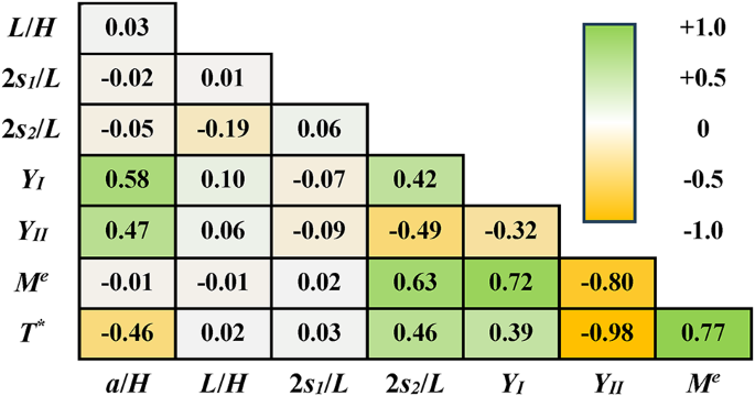
Heatmap of the dataset and the values of correlation.

Figure 4 shows histograms for each output variable, with a kernel density estimation (KDE) curve overlay offering a smoothed probability density function representation. As can be seen in these figure, the distribution of data is not follow any common distribution function, as Y_I and Y_II parameters only can be positive values, a great positive skewness was seen for them, while the skewness of the T* data is highly negative. Also for Y_II and T* the kurtosis is significant. Figure 5 presents the quantile-quantile (Q-Q) plots comparing the observed data’s empirical quantiles with the theoretical quantiles of a standard normal distribution. Points near the diagonal line indicate approximate normality, while deviations suggest a lack of it.

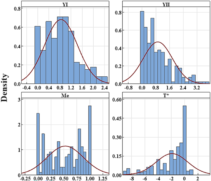
Distribution of geometry factors and their comparison with normal distribution.

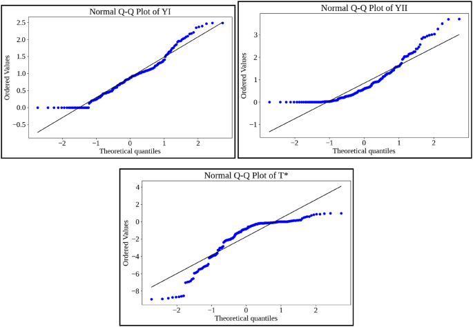
Q-Q plot of the output parameters of the ASENB dataset.

Machine learning algorithms exhibit varying degrees of sensitivity to feature scaling and distributional characteristics, potentially impacting model performance. These distributional properties can negatively influence the training process, particularly for algorithms sensitive to feature scaling, leading to suboptimal performance.

To mitigate these potential issues, we employed min-max normalization across all features. This technique scales all feature values to a range between 0 and 1, effectively addressing differences in magnitude and, to some extent, reducing the impact of skewness and kurtosis. While min-max normalization does not completely eliminate skewness, it standardizes the feature scales, preventing features with larger values (potentially due to skewness or outliers) from dominating the learning process. This is particularly crucial for Bidirectional Long Short-Term Memory networks (BiLSTMs), which are known to be sensitive to feature scaling and benefit from normalized inputs to avoid training instability and performance loss.

The min-max normalization was applied after dividing the dataset into training, validation, and testing sets (by a ratio of 60%, 20%, and 20%, respectively) to avoid data leakage, ensuring the integrity of the model evaluation. While further investigation into alternative normalization techniques specifically designed to address skewness (e.g., power transforms, Box-Cox transformation) could potentially yield further improvements, the min-max normalization provided a robust and computationally efficient method for standardizing feature scales and improving the overall reliability and performance of our machine learning analysis.

Regression

Regression analysis assumes a relationship between the variables, which can be represented mathematically. In its simplest form, where the relation of an output and several inputs was sought, the multiple linear regression (MLR) can be used. MLR in its simple form evaluates the linear relations between inputs and outputs without considering the classification of outputs based on one or more input variables (Eq. 8).

As a more descriptive model, in MLR, the outputs can be evaluated in classifications. In these cases, the outputs were separate based on a variable (Eq. 9). This framework is usually named multiple linear regression with classification of outputs (MLRC).

For datasets with non-linear trends or those where the interatom of variables may affect the trends, the inputs with higher terms or the interaction of inputs should also be included (Eq. 10), known as polynomial regression (PR).

Also considering classifications of outputs in PR model (PRC) can increase the accuracy of presented mathematical models (Eq. 11).

In these equations, y is the dependent variable, the outcome we are determined to predict. The term \(\delta\) is the y-intercept of the regression line. \({\beta _1}\), \({\beta _2}\), \({\beta _n}\) are the coefficients of the independent variables \({x_1}\), \({x_2}\), and \({x_n}\). \(\varepsilon\) represents the error term, which captures the difference between the predicted and actual values. i shows the class of the output regarding the classification of output.

Random forest regression

Random Forest Regression is an ensemble learning approach that identifies non-linear relationships among variables (Fig. 6). Each tree is trained on a random subset of the data, enhancing diversity and mitigating overfitting. The overall prediction is the average of the predictions made by these trees³⁶. In RFR, the final prediction is computed as Eq. (12).

Where \({T_i}\). represents the prediction made by the \(i – th\) tree in the decision forest, this output is generated based on the input vector \({T_i}\). The symbol N represents the total number of decision trees included in the forest, which collectively contribute to the overall prediction process. The final prediction, denoted as \(\hat {Y}\), is calculated by taking the average of the predictions.

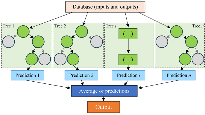
RFR Flowchart used to predict mode I/II brittle fracture parameters.

Bidirectional long short-term memory deep learning model

BiLSTMs are deep learning models specifically created to capture long-term dependencies in sequential data. A BiLSTM network consists of two separate layers that work simultaneously. The Forward Pass processes the input sequence from start to finish, capturing historical trends and relationships. In contrast, the Backward Pass processes the sequence in reverse, enabling the model to predict future trends and behaviors. The operations of an LSTM unit are defined as Eq. (13)^37,38,39.

Equation (13) (forget gate) determines which information to discard from the previous state. Where, \({f_t}\) is forget gate activation, \(\sigma\) is a sigmoid activation function (produces output between 0 and 1), \({W_f}\) is the weight matrix for the forget gate, \({h_{t – 1}}\) is the hidden state from the previous time step, \({x_t}\) is input at the current time step, and \({b_f}\) is Bias for the forget gate. Equations (14) and (15) decide which new information to store (Input Gate).

Where, \({i_t}\) is input gate activation, \(\widetilde {{{C_t}}}\) is candidate cell state (represents the potential new information to be stored in the cell state), and \({\text{tanh}}\) is hyperbolic tangent activation function (outputs values between − 1 and 1). In this condition the cell state update using Eq. (16).

Where, \({C_t}\) is the memory of the network, updated by combining the forget gate and input gate activations. Equations (17) and (18) decides the part of the cell state to output at the current time step.

Where, \({O_t}\) is output gate activation.

It is important to note that the equations presented for the BiLSTM results are not the intrinsic governing equations of the neural network. BiLSTM models operate as black-box frameworks, where predictions are generated through sequential nonlinear transformations of hidden states. Such processes do not yield closed-form analytical expressions. To improve interpretability and facilitate practical engineering use, we applied symbolic regression to the BiLSTM outputs. The resulting equations, therefore, act as surrogate regression forms, approximating the predictive behavior of the trained BiLSTM while offering transparency and analytical tractability. These symbolic expressions should be viewed as interpretable approximations rather than direct representations of the BiLSTM architecture.

Figure 7 presents a flowchart outlining the BiLSTM technique employed in this study.

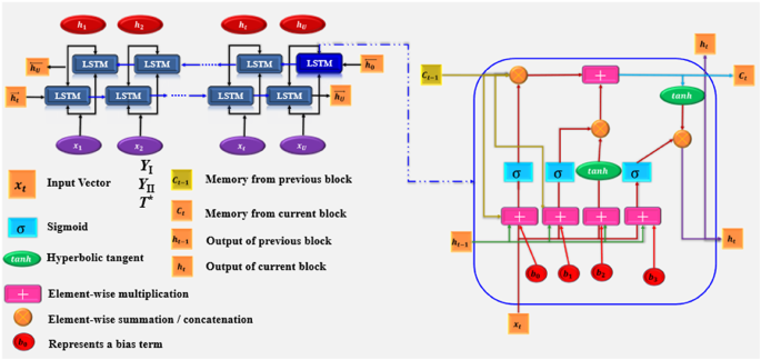
BiLSTM Flowchart used to predict mode I/II brittle fracture parameters.

Hyperparameter tuning (layer size, tree depth, loss function) was performed using a trial-and-error approach, testing 50 sets of parameter values per model with 5-fold cross-validation on the training set to optimize model performance and prevent overfitting. Therefore, this study’s BiLSTM network consisted of 5 LSTM units, a learning rate of 0.001, a batch size of 16, and a training duration of 200 epochs. To prevent overfitting, a dropout rate ranging from 0.2 to 0.5 was incorporated into the BiLSTM layers. Furthermore, early stopping was implemented during BiLSTM training, monitoring the validation loss and halting training when the loss failed to improve for 10 epochs. This ensured that the model did not continue to train and memorize the training data beyond the point of optimal generalization. L1 regularization was tested but did not improve results and increased computational cost, so was not incorporated into the final model.

The RFR model was configured with 100 trees, a maximum depth of 7, a minimum sample split of 2, and a minimum sample leaf of 3. Moreover, the BiLSTM model was first trained on time-series data to capture complex, nonlinear dependencies between input sequences and target outputs. Once trained, the model’s predictions, representing the learned relationships, were used as the target data for a Symbolic Regression (SR) process. The SR algorithm, implemented via Genetic Programming, searched for a compact analytical expression that approximates the BiLSTM’s predictive behavior. The resulting equation, composed of mathematical operators and functions (e.g., sin, cos, log, and power terms), serves as an interpretable surrogate model that mirrors the BiLSTM’s outputs without exposing its internal computational architecture. This approach bridges the gap between high-performance black-box deep learning models and the need for transparent, physics-consistent analytical forms in engineering applications.

In addition to the BiLSTM and RFR models, a Multilayer Perceptron (MLP) method was employed to refine the modeling process further. The MLP architecture consisted of 3 hidden layers, each containing five neurons, and a trial-and-error approach was used to identify the optimal combinations for training and testing the models. Similarly to the BiLSTM, the MLP also incorporated early stopping based on validation loss and L2 regularization to prevent overfitting. All the models were trained in a multi-output configuration, enabling the prediction of all three target parameters simultaneously and simultaneous learning of correlated features. This demonstrated that performance differences were negligible (change in RMSE < 1%) compared to individual-output training. So, in order to minimize the computational complexity, a same configurations were utilized for all outputs.

Model performance evaluation metrics

To evaluate the reliability and accuracy of predictive models, a range of performance metrics was utilized, including the coefficient of determination (R²), root mean square error (RMSE), mean absolute error (MAE), and standard deviation (SD) of prediction errors. Results and discussion.

Sensitivity analysis

The Morris method, as a global sensitivity analysis, was used as the first step in evaluating the possible relationship between input variables and output results. The Morris method calculates elementary effects by varying one input parameter at a time while keeping others constant, allowing identification of parameters that have linear, nonlinear, or interaction effects. A trajectory-based sampling approach was employed, generating multiple random paths in the space. For each path, one parameter was perturbed by a fixed step size (Δ), and the corresponding change in the output was recorded. The elementary effect (EE) was computed for each parameter as Eq. (19).

where y represents the model output, and k is the number of input parameters. The mean (µ) and standard deviation (σ) of the elementary effects were calculated for each parameter to quantify its overall influence and the degree of nonlinearity or interactions, respectively.

Following the screening of the Morris method, the Sobol method performed a more detailed sensitivity analysis. The Sobol method quantifies the contribution of each input parameter to the output variance, including both individual and interaction effects (total-order indices). The results of the Morris and Sobol analysis are summarized in Table 3.

As can be seen in Table 3, the 2S₂/L ratio exhibits the highest mean effect (µ = 1.85) with low standard deviation (σ = 0.12), indicating a strong and consistent influence on the outputs. a/H shows a mean moderate impact (µ = 1.20) with slightly higher standard deviation (σ = 0.18), suggesting some nonlinearity or interactions. L/H has a lower mean effect (µ = 0.95) but higher standard deviation (σ = 0.22), implying potential nonlinear effects or interactions with other parameters. 2s₁/L demonstrates the lowest influence (µ = 0.10, σ = 0.05), making it the least significant parameter. The results of the Morris method were also checked with the Sobol analysis, and there was good agreement.

Although the sensitivity analyses indicated that 2S₁/L parameter exhibited the lowest influence on output variance, it was retained in the modelling. This decision was made for several reasons: (i) 2S₁/L is a fundamental geometric ratio in defining the ASENB configuration, and its exclusion would render the problem formulation incomplete; (ii) the parameter may still participate in nonlinear interaction effects with other variables; (iii) narrow variation range of 2S₁/L in the dataset (0.7–0.9) inherently reduces its observed sensitivity, whereas broader ranges could reveal stronger effects; and (iv) retaining it ensures consistency with prior fracture mechanics studies and avoids introducing bias in the machine learning models by pre-eliminating geometric descriptors. .

Geometry factors estimations

Multiple and polynomial regression

Scatter plots were applied to two datasets by comparing actual versus predicted values for four regression models (MLR, MLRC, PR, and PRC), as denoted in Fig. 8. The results show that all the models have R² values lower than 0.66. The MLR, as the simplest regression model, can model the data with R² values of about 0.45, which is unacceptable. The accuracy of the MLRC model also did not improve. Taking the interactions between the inputs and considering their quadratic effects improves the accuracy of the data, raising R² to about 0.66; however, this accuracy is not acceptable. As discussed and seen in other studies, the relationships between fracture parameters exhibit high nonlinearity; consequently, the linear regression employed here is insufficient to fully capture the complexities of these equations, resulting in the observed scatter in the predicted values. Therefore, a pressing need exists for developing and applying more sophisticated modeling techniques to handle this complexity^40,41,42.

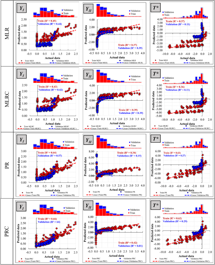
Scatter plot of the correlation-based input distribution and predicted fracture characteristics using MLR, MLRC, PR, and PRC models.

Random forest regression (RFR)

This section presents the results obtained from the RFR technique for predicting the fracture parameters Y_I, Y_II, and T^*. These models utilized dimensionless aspect ratios, detailed in Table 1, as input variables, representing the geometric characteristics of the system under investigation. The resulting model equations, derived from the RFR technique, are provided in Table 4. This table explicitly illustrates the relationship between the input dimensionless parameters and the predicted fracture toughness values, offering a quantitative representation of the developed predictive models.

Equation (20) exemplifies the form of the equations generated by the RFR model’s prediction of Y_I. The intercept term, represented as “1.48,” indicates the predicted value of Y_I when all independent variables approach zero. The independent variables\(\:-(L/H),\:(2{S}_{2}/L),\:(a/H),\:(2{S}_{1}/L)-\)are dimensionless geometric parameters that characterize the system under investigation. The terms “\(\:(-0.242/(L/H\left)\right)\)” and “\(\:(-0.214/((L/H)(2{S}_{2}/L)\left)\right)\)” reveal an inverse relationship between Y_I and these features; as \(\:(L/H)\) increases, the contribution of these terms diminishes, indicating a negative correlation. Likewise, an increase in \(\:(2{S}_{2}/L)\) leads to a reduction in the influence of the second term. The complexity of the equation is further highlighted by the term “\(\left( {9.02\left( {a/H} \right)^{2} cos\left( {\left( {2S_{1} /L} \right)} \right)} \right)^{{1.08}}\),” which suggests a non-linear relationship between Y_I and the independent variables. This term involves squaring \(\:(a/H)\), applying the cosine function to \(\:(2{S}_{1}/L)\), and raising the result to the power of 1.08, indicating a relationship that, while close to linear, retains non-linear characteristics. The introduction of the cosine function implies cyclical behavior, suggesting that the effects of these parameters may vary periodically. Additionally, the term “\(\:-3.9(a/H)cos\left(\right(2{S}_{1}/L\left)\right)\)” demonstrates another non-linear interaction involving both \(\:(a/H)\) and the cosine of \(\:(2{S}_{2}/L)\), with the negative sign indicating a detrimental contribution to Y_I.

Figure 9 presents a comparative evaluation of the performance of the Random Forest Regression (RFR) models in predicting concrete fracture parameters. The scatter plots illustrate the relationship between the predicted values generated by the models and the actual measured values. The red data points in these plots represent the training dataset, while the blue points correspond to the validation dataset. The histograms positioned above each scatter plot provide additional insight by displaying the distribution of the predicted values. Notably, the histograms reveal greater dispersion in the validation data compared to the training data, which is expected since the validation data represents unseen inputs that the model must predict without prior exposure. This dispersion serves as an indicator of the model’s generalization capability and its ability to handle new data.

The scatter plots demonstrate a generally positive correlation between the predicted and actual values, as evidenced by clustering data points around the diagonal line. This alignment suggests that the models are reasonably accurate in their predictions. However, the slight deviations observed, particularly in the validation data, highlight the inherent challenges in predicting complex fracture parameters. These deviations may arise from the data’s nonlinear nature or the model’s limitations in capturing all underlying patterns. The results indicate that the RFR models perform well in predicting concrete fracture parameters, with a strong correlation between predicted and actual values. This step is crucial in validating the models’ reliability and ensuring their applicability to real-world scenarios, where accurate predictions of material behavior are essential for structural integrity and safety.

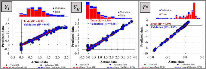
Plot of the correlation-based input distribution and predicted fracture characteristics for RFR.

Bidirectional long Short-Term memory networks (BiLSTMs)

The results of the Bidirectional Long Short-Term Memory (BiLSTM) model are presented in Table 5. Equation (25), like Eq. (20), represents a nonlinear regression equation generated to predict the fracture toughness parameter (but here for T^*). The equation’s complexity highlights the intricate relationship between T and the dimensionless geometric parameters \(\left( {a/H} \right)\), \(\left( {L/H} \right)\), \(\left( {2S_{1} /L} \right)\), and \(\left( {2S_{2} /L} \right)\). Unlike a simple linear model, Eq. (25) incorporates several nonlinear terms and interactions, indicating that the influence of each parameter on T^* is not additive. The constant term, -1.47, represents the predicted value of T^* when all independent variables are zero. The term \(3.39~\left( {a/H} \right)\) shows a positive linear relationship between T^* and (a/H). In contrast, the term \(\left( { – 1.02/\left( {\left( {L/H} \right)\left( {2{S_2}/L} \right)} \right)} \right)\) demonstrates an inverse relationship; increasing \(\left( {L/H} \right)\) or \(\left( {2S_{2} /L} \right)\) decreases T^*. The most complex component is the large fractional term, which contains multiple nested functions, raising \(\left( {0.567~ – ~0.407\left( {15.1\left( {a/H} \right)} \right)^{{\left( {\left( { – 0.655\left( {L/H} \right)} \right)/\left( {15.1\left( {a/H} \right)^{3} ~ + ~\left( {L/H} \right)\left( {2S_{1} /L} \right)^{2} } \right)} \right))}} } \right)\) to a power that itself is a function of \(\left( {a/H} \right)\) and \(\left( {L/H} \right)\). This highlights significant non-linear interactions and dependencies between multiple input parameters. The presence of exponentiation and division within this fractional component indicates that the influence of each parameter is not simply additive but rather depends on the values of the other parameters. In summary, while Eq. 22 shows some non-linear effects, Eq. (25) reveals a far more complex and highly nonlinear relationship between the predictor variables and T^*, underlining the limitations of simpler linear models for this prediction task.

BiLSTM shows a reasonable fit (Fig. 10) but has a slightly less accurate of the validation data compared to RFR. The scatter plot displays more spread, especially in the validation set, and the difference between the training and validation R² values indicates a degree of overfitting, though less severe than RFR. The crucial distinction is the model’s ability to generalize to new, unseen data. BiLSTM consistently performs across the training and validation sets, whereas RFR shows a more significant discrepancy, suggesting overfitting, particularly for RFR.

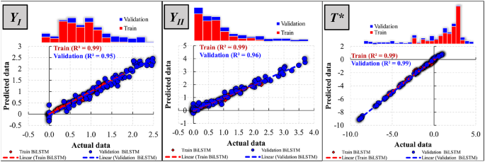
Scatter plot of the correlation-based input distribution and predicted fracture characteristics for BiLSTM.

Comparative analysis of machine learning (ML) model performance

The performance of models in predicting the parameters was evaluated using statistical indicators. The models were assessed across the training and validation phases. Random Forest Regression (RFR) performed strongly during the training and validation phases. In training, RFR reached an R² value of 0.99 for Y_I and 0.99 for Y_II, signifying a high level of variance explained by the model. The RMSE and MAE values were low (0.032 and 0.016 for Y_I, respectively), indicating accurate predictions. In the validation phase, the R² values remained high (0.93 for Y_I and 0.96 for Y_II), although slightly lower than those in the training phase. The RMSE and MAE increased (0.203 and 0.144 for Y_I), reflecting a drop in accuracy when predicting unseen data. Despite this, RFR demonstrated strong performance, highlighting its reliability in interpolation and extrapolation scenarios.

Bidirectional Long Short-Term Memory (BiLSTM) also performed well across both phases. During training, BiLSTM achieved R² values of 0.99 for Y_I and 0.99 for Y_II, with RMSE and MAE values slightly higher than RFR but still indicating good predictive capability. In the validation phase, the model maintained high R² values (0.95 for Y_I and 0.96 for Y_II) and relatively low RMSE and MAE (0.175 and 0.136 for Y_I), demonstrating its robustness in extrapolation. This consistent performance highlights BiLSTM’s effectiveness in handling complex datasets and making accurate predictions on unseen data.

In contrast, Multiple Linear Regression (MLR) and MLR with Classification (MLRC) showed limited predictive power. During training, both MLR and MLRC exhibited lower R² values (0.45 for MLR and 0.43 for MLRC for Y_I) and higher RMSE and MAE, indicating a poorer fit compared to RFR and BiLSTM. In the validation phase, the performance further degraded, with R² values dropping to 0.44 for MLR and 0.43 for MLRC for Y_I. This decline underscores the limitations of these models in both interpolation and extrapolation scenarios, suggesting that they may not be suitable for complex predictive tasks.

Polynomial Regression (PR) and PR with Classification (PRC) exhibited moderate performance during the training phase, with R² values of 0.64 for PR and 0.66 for PRC for Y_I. However, the RMSE and MAE were higher than those of RFR and BiLSTM, indicating less accurate predictions. In the validation phase, the models showed a significant drop in R² values (0.57 for PR and 0.64 for PRC for Y_I), further highlighting their reduced predictive power when applied to validation data. This suggests that while PR and PRC may perform adequately within the training data range, their effectiveness diminishes when extrapolating to new data.

For the T^*, RFR and BiLSTM continued to perform strongly. During training, RFR achieved an R² value of 0.99, with low RMSE and MAE values (0.131 and 0.1004, respectively). In the validation phase, the R² value slightly increased to 0.99, with RMSE and MAE values of 0.127 and 0.092, respectively. This indicates that RFR maintained high accuracy and consistency even when applied to the T^* dataset. Similarly, BiLSTM performed well during training with an R² value of 0.99 and RMSE and MAE values of 0.142 and 0.088, respectively. In the validation phase, BiLSTM achieved an R² value of 0.99, with RMSE and MAE values of 0.122 and 0.1006, respectively. These results further confirm the robustness of RFR and BiLSTM in handling different datasets.

On the other hand, MLR and MLRC showed poor performance on the T^*. MLR had an R² value of 0.37 during training, with high RMSE and MAE values (2.107 and 1.729, respectively). In the validation phase, the R² value dropped to 0.11, with RMSE and MAE values of 1.025 and 0.807, respectively. MLRC exhibited similar trends, with an R² value of 0.36 during training but a significant drop to 0.11 in the validation phase. PR and PRC also struggled, with R² values dropping from 0.61 to 0.62 during training to 0.27289 and 0.29916 during validation, respectively. These results highlight the limitations of simple regression methods in accurately predicting the failure parameters for the T^* dataset.

RFR and BiLSTM outperformed the simple regression methods (MLR, MLRC, PR, PRC) in interpolation and extrapolation scenarios, as evidenced by their higher R² values and lower RMSE, MAE, and SD. These results suggest that machine learning and deep learning models are more powerful and reliable for predicting the parameters of mode I/II brittle fracture of single-edge notched bend specimens, mainly when dealing with unseen data. While computationally less intensive, the simple regression methods showed limited predictive power, especially in extrapolation tasks. This analysis underscores the importance of selecting appropriate modeling techniques based on the data’s complexity and the predictive task’s specific requirements. Model performance across two datasets was shown in Table 6.

The marginal performance advantage of BiLSTM over RFR in certain validation cases can be attributed to BiLSTM’s ability to capture bidirectional dependencies within sequential patterns of the fracture data, enabling it to learn subtle temporal or path-related relationships that tree-based ensemble methods cannot explicitly model. This advantage becomes more pronounced when the predictive task involves extrapolating patterns beyond the range of training samples, particularly in scenarios where the fracture behavior exhibits cumulative or history-dependent effects. However, RFR remains highly competitive and in some cases matches or slightly outperforms BiLSTM, especially when the relationships are predominantly nonlinear but not strongly sequential. In practice, BiLSTM may be preferred when the dataset exhibits ordered, interdependent features or when extrapolative robustness is essential, whereas RFR offers an effective and computationally efficient choice for high-dimensional, heterogeneous tabular data with limited sequential structure. The complementary strengths of both models suggest that the choice between them should be guided by the underlying data characteristics and the intended application context.

Figure 11 shows a Taylor diagram comparing machine learning models’ performance predicting parameters Y_I, Y_II, and T^*. It analyzes the entire dataset using standard deviation (radial distance) and correlation coefficient (angular position) to assess accuracy and precision. Points near the reference indicate better performance, with closer radial distances showing lower predictive variability and higher precision. A correlation coefficient near 1 suggests strong agreement with actual measurements. For instance, BiLSTM has a high correlation with actual measurements but a larger standard deviation than RFR, indicating greater prediction variability despite good agreement.

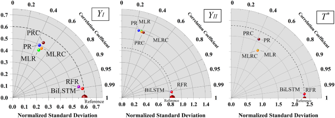
Taylor Diagram for Evaluating the Performance of ML Models. (A) Y_I, (B) Y_II, and c) T^*.

Figure 12 shows SHAP analyses (SHapley Additive exPlanations) of feature importance and their impact on XGBoost model predictions. The left column features dot plots illustrating SHAP values across all instances. Each dot’s horizontal position indicates the feature’s contribution, placing on right side means positive impact (increasing predictions), and placing on left side means negative (decreasing predictions). The dot color represents feature value magnitude, from low (dark blue) to high (dark red), visualizing relationships between feature value and impact. For example, a/H shows a positive impact at higher values and inconsistent effects at lower values, while 2s₂/L shows a negative impact at higher values. This analysis highlights the importance of features and their influence on Y_I prediction. The right column contains heatmaps displaying SHAP values for each feature across individual instances, providing detailed insights into feature influence. The color scale ranges from negative (blue) to positive (red), with the top panel showing individual predictions and variability. The heatmaps reveal significant heterogeneity in feature impact; for instance, a/H has a strong positive effect in some cases but little or negative impact in others, illustrating the complexity of feature relationships and the model’s capacity to capture these non-linear interactions. Combining dot plots and heatmaps from SHAP analyses offers a granular understanding of feature contributions to XGBoost predictions, enhancing traditional metrics by revealing overall importance and variability across instances, leading to a comprehensive assessment of model behavior and prediction drivers.

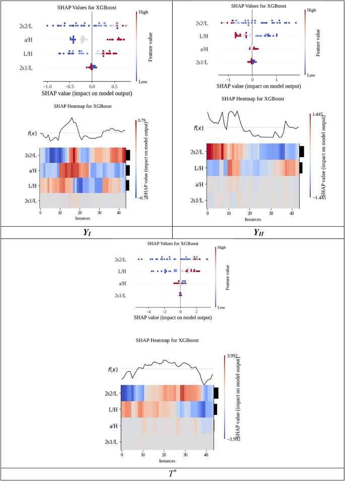
Interpreting the influence of input parameters on fracture predictions using SHAP.

The SHAP analysis and Taylor diagram together provide end-to-end model performance evaluation. The Taylor diagram shows correlation, standard deviation, and RMSE on one graph, with both accuracy and prediction consistency; i.e., BiLSTM shows high conformity with observed data but greater variability than RFR. SHAP analysis complements this by quantitatively measuring feature contributions, expressing how each feature contributes positively or negatively to predictions, and detecting potentially overlooked non-linear interactions. Together, these tools enhance interpretability by facilitating a better comprehension of model behavior, drivers of prediction, and relative strengths of each machine learning approach.

As the machine learning method again proved to be accurate in mechanical engineering, particularly here in predicting fracture parameters, the practical implications of this study are twofold. First, the results demonstrate that advanced data-driven models such as RFR and BiLSTM networks can provide highly accurate predictions of fracture parameters at a fraction of the computational cost of FEM analyses. A single FEM simulation typically requires the generation of a detailed mesh, singular crack-tip elements, and convergence testing, often amounting to hours for each geometry. In contrast, once trained, the machine learning models can produce predictions in milliseconds with negligible computational resources. This efficiency makes them particularly advantageous for parametric studies, real-time applications, and large-scale optimization problems where thousands of geometry–loading configurations must be evaluated. Second, from an engineering practice perspective, the proposed models provide a practical alternative for design, reliability assessment, and preliminary screening of structural configurations. Engineers can employ the trained models to rapidly estimate fracture parameters without resorting to repeated FEM analyses, thereby accelerating the decision-making process.