
Batch evaluation of collective owned commercialised construction land using machine learning

RF land value bulk assessment model construction
Constructing a batch appraisal system for CCCL prices using RF depends on fine-tuning model parameters, including the number of decision trees, the feature selection method, and the depth of the trees. Through iterative training and validation, the model was optimised to achieve a high degree of fit on the training set while demonstrating strong predictive accuracy on the test set. Once training was complete, the core parameters and model structure were saved, enabling its application to the feature data of the parcels to be appraised, thereby achieving batch appraisal.
The RF land price model based on R, after variable selection, was primarily influenced by two factors: the number of variables selected for the decision tree bifurcation nodes (mtry) and the number of decision trees used for training and prediction in the RF (ntree). The mtry parameter determines the number of variables considered for each binary split in the decision trees of the RF model, while ntree represents the number of decision trees used for training and prediction. In this study, mtry was set to 5 and ntree to 500. These parameter values were selected based on two considerations. First, the characteristics of the data and the attributes of the appraisal objects were carefully evaluated. Specifically: (1) Feature dimensionality suitability: Thirteen feature factors were used in this study (X1-X13). According to the original design of the RF model, the default value for regression tasks was p/3 ≈ 4.33. Rounding this up to 5 follows theoretical convention. Under this condition, RF can retain sufficient information (avoiding high bias from using too few features) while mitigating feature collinearity (e.g., potential spatial correlation between X5, road accessibility, and X6, external transportation convenience) through random sampling. (2) Data characteristics suitability: CCCL market entry encompasses diverse types, requiring the model to capture nonlinear interaction effects (e.g., the interaction between X12, market entry approach, and X13, planned use). Moderately increasing mtry above the default value of 4 enhances the expressive power of individual trees while avoiding overfitting. (3) Convergence assurance: CCCL is characterised by “small parcel size and large quantity”, leading to significant data noise. Setting ntree to 500 ensures sufficient error convergence, preventing small-sample noise from interfering with the model’s generalisation ability.
Second, the parameter selection was also based on parameter testing and optimisation. The parameter mtry determines the number of variables for each bifurcation in the decision trees of the RF model, while ntree is the number of decision trees used for training and prediction. In this study, the optimal mtry value was determined using the following steps: (1) Set the ntree value to 200, vary mtry from 1 to 13, and perform modelling 13 times to obtain the corresponding goodness-of-fit results. (2) Set the ntree value to 500, repeat the steps in (1), and repeat the above operation in increments of 500 trees. This was repeated until there was no obvious change in the model’s goodness-of-fit curve. The training results are shown in Fig. 3, where the model achieves maximum goodness-of-fit when the mtry value is around 5, and the curves are more concentrated. Therefore, this study adopted the mtry value of 5 as the optimal parameter.

Model goodness of fit versus mtry value.
Based on the R software, the mtry value was set to 5 to explore the relationship between the residual sum of squares and the number of ntree of the RF model, and the graph of their quantitative relationship is shown in Fig. 4.
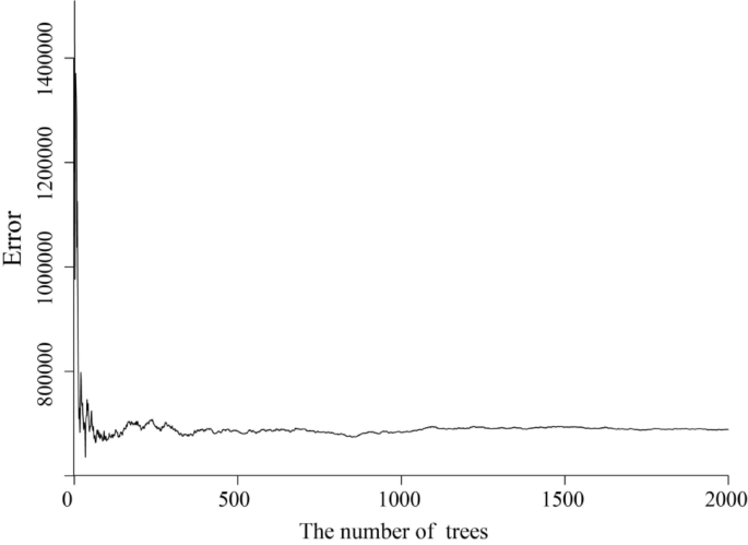
Model residual sum of squares versus ntree values.
Figure 4 shows that the model tends to stabilise when the ntree value exceeds 500. Therefore, this study set the ntree value to 500 as the final optimised parameter. The parameters of the RF land price batch appraisal model are shown in Table 2.
BPNN land value bulk evaluation model construction
The BPNN was used to conduct batch appraisal of CCCL prices. This required repeated adjustments to key parameters including the activation function, training function, training target error, and the maximum number of training iterations. This continued until the training set fit test was qualified, and through the prediction set accuracy test, the training could be ended to save the network weights and the queue value matrix, and to enter the characteristics of the parcel to be evaluated for values for the bulk assessment of CCCL.
This study selected 13 model variables for CCCL batch appraisal. Consequently, the input layer of the BPNN model contained 13 nodes. The output layer, representing the CCCL market-entry price, had one node. Based on this, and through the application of empirical formulas combined with grid search validation, the number of hidden layer nodes was set to 21. This configuration maintained the nonlinear modelling capabilities while avoiding overfitting. The network architecture comprised three layers: input, hidden, and output layers. The key parameter settings for constructing the BPNN-based batch appraisal model for land prices are presented in Table 3.
SVM land value bulk assessment model construction
This study was based on the MATLAB software, using the libsvm-mat-2 [1]0.89 − 3 [FarutoUltimate3.0Mcode] version of the toolbox to perform model training and prediction. The dataset comprised a training set of 102 samples and a test set of 16 samples. The mapminmax function in MATLAB 2018a was used for normalisation, followed by data transposition before inputting the data into the SVM model. Regarding the choice of kernel function, due to the current lack of research on CCCL market entry indicators in China and the absence of prior knowledge about the data, this study employed the Radial Basis Function (RBF) kernel, known for its smoothing properties, as the kernel function for the SVM model. When the SVM prediction is a smooth estimate, the computational cost is reduced while maintaining good predictive performance. The key SVM parameters, penalty (C) and kernel (gamma), were selected based on both theoretical and empirical considerations, with final values of 32 and 0.1768, respectively. On the one hand, these values were obtained through optimisation using a mesh grid search. On the other hand, the CCCL market is subject to policy intervention noise (e.g., administrative directives on the market entry approach, X12). A higher penalty value allows for the misclassification of a small number of outliers, which prevents overfitting and avoids an overly lenient model (e.g., underfitting in the training set when C < 10). Using standardised data, the theoretically optimal kernel value was 1/(13 × average variance). Given the substantial proportion of land-related indicators in the indicator system, and considering that the variance of these indicators after scaling often falls between 0.2 and 0.6, taking the average variance as 0.4 yielded a theoretically optimal kernel of 0.1923. A reasonable kernel parameter should be close to this value. The specific model parameter settings are shown in Table 4.
Comparison of forecast results
Currently, the number of collective operating land transactions in Beiliu City is limited, and the characteristics of the traded land vary widely. To ensure the comprehensiveness of the bulk assessment model, the representative characteristics of the traded objects should be thoroughly selected as test samples. Among the 118 CCCL transaction samples in Beiliu City’s, there are four market-entry methods: in-situ entry, remediation entry, adjustment entry, and entry after approval for agricultural land conversion to new construction land. There are five planned uses for entering the market: industrial and mining land, public administration and public land, commercial land, and commercial and residential land; and five planned uses for the samples. The transaction samples can be classified by entry zones, including Beiliu Town (the outskirts of Beiliu City), Dali Town (suburbs), Dali Town (the north of Beiliu City), Beiliu Town (suburb of Beiliu City), Dali Town (northwestern part of Beiliu), Liujing Town (southern part of Beiliu), Longsheng Town (central part of Beiliu), Minan Town (eastern part of Beiliu City), Qingshuikou Town (central part of Beiliu), Tangshi Town (southwestern part of Beiliu), and Xinweizhen Town (northwestern part of Beiliu), and other major areas. The 16 sample parcels selected for the test set, based on the four characteristics of market-entry time, market-entry location, market-entry use, and market-entry route, along with the absolute error of the model’s predictions, are shown in Table 5.
Based on the results presented in Table 5, we conducted a detailed analysis of the prediction accuracy of the machine learning models for CCCL market-entry prices. The absolute prediction errors in the table revealed significant variations in the performance of different models across different land-use types and regions. First, RF exhibited a relatively balanced predictive performance across all land use types, particularly for commercial residential land, industrial mining warehousing land, and residential land, where its errors are relatively small, demonstrating an advantage over other models. By contrast, the BPNN showed greater fluctuations in prediction errors, suggesting that it may struggle to capture accurate predictions in certain complex nonlinear relationships. The SVM performed poorly in some areas with high market uncertainty, possibly because it struggles to capture more nuanced price variation patterns. From a geographical perspective, the prediction errors for the CCCL market-entry prices in the western and suburban areas of Beiliu City were generally higher.
This trend was particularly evident in the predictions of the BPNN and SVM models, indicating that the RF still possesses a degree of adaptability when dealing with these complex markets. Furthermore, for newly developed areas, larger prediction errors may stem from incomplete data, as these areas have not yet established stable market trends. Examining different market-entry approaches, variations in land prediction errors reflect the uncertainty of market information and the complexity of land policies. “On-site market entry” land exhibited smaller prediction errors due to the relative stability of the market and clearer information; however, “adjusted market entry” and, especially, “consolidated market entry” land showed larger prediction errors due to the complexity of policy changes and market adjustment periods. Therefore, the performance of prediction models varied significantly across different land market entry approaches. For “consolidated market entry” land, in particular, more market data and policy background information are needed to improve prediction accuracy. Looking at the individual test samples, Samples 6, 7, 9, 12, and 16 in the test set showed greater dispersion between the model’s predicted values and the actual values (Fig. 6), indicating a larger deviation between the model’s overall prediction results and the true values. According to Table 5, the market entry time for Sample 6 and the subsequent samples was three years or later after the policy pilot, and their errors were significantly higher than those in the early stages of policy implementation.

Comparison of true and predicted values of the training set.
Figures 5 and 6 show that the RF, BPNN, and SVM models exhibited varying predictive capabilities when forecasting CCCL prices. RF demonstrated a relatively stable fit to the training set, and the fluctuations in its predicted values aligned with those of the actual values, indicating that RF has a good ability to capture the underlying trends in the data. The training set error was relatively small, particularly in areas with more volatile price fluctuations. For the test set, the RF model maintained relatively stable predictions that closely matched the fluctuations in the actual values. This demonstrates good generalisation ability and predictive accuracy, effectively reducing overfitting and maintaining good performance in predicting new data. The BPNN exhibited a relatively smooth fitting curve for the training set. Although deviations were observed in the predicted values for certain peaks and troughs, the overall trend was relatively accurate. The BPNN can predict more accurately in areas with fewer price fluctuations, but in areas with significant price fluctuations (as seen in the middle section of Figure b), its prediction errors increase significantly, showing some signs of overfitting. For the test set, the BPNN prediction errors were relatively large, particularly in areas with significant price fluctuations where the difference between the model’s predictions and actual values was more pronounced. This suggests that the BPNN may be affected by overfitting when dealing with complex market fluctuations and is more sensitive to local changes. The SVM prediction results were relatively consistent with the fluctuations in the actual values. However, compared with the RF and BPNN, the SVM’s fitting curve appears smoother and fails to accurately capture drastic price changes in some highly volatile areas. This reveals SVM’s limitations when dealing with highly volatile data, possibly because its implicit assumption of linearity does not adapt well to the nonlinear characteristics of the data. The SVM’s performance was slightly inferior to those of the RF and BPNN, especially in test set intervals with significant price fluctuations, where there was a larger deviation between the SVM’s predictions and actual values.

Comparison of predicted results and real values.
Precision comparison
To test the simulation accuracy of the three models, this study selected R2, RMSE, MAE, and RA as evaluation metrics. R2 represents the degree of fit between the predicted and actual results; the closer R2 is to 1, the better the model prediction effect. RMSE measures the deviation between predicted and actual values, while MAE is the mean absolute error. MAE is less sensitive and more inclusive than the outlier samples, meaning smaller RMSE and MAE values indicate more accurate prediction results. RA indicates the degree of proximity between the predicted quantity and the actual situation, the higher the RA, the more accurate the prediction. Detailed results of the accuracy test are shown in Table 6.
As shown in Table 6, the model fit (R²) of RF, BPNN, and SVM in the training set was 96.6%, 89.0%, and 93.8%, respectively; the root mean square error (RMSE) was 17.8 RMB, 24.1 RMB, and 22.9 RMB, respectively; the mean absolute error (MAE) was 14.8 RMB, 20.4 RMB, and 18.2 RMB, respectively; and the prediction accuracy (RA) was 96.6%, 92.5%, and 95.6%, respectively. In the test set, the R² values for RF, BPNN, and SVM were 90.42%, 83.29%, and 86.63%, respectively; the RMSE was 21.37 RMB, 30.23 RMB, and 28.11 RMB, respectively; the MAE was 17.50 RMB, 25.58 RMB, and 24.26 RMB, respectively; and the prediction accuracy RA was 94.77%, 91.21%, and 91.94%, respectively.
In summary, among the three machine learning models used for the price assessment of Beiliu City’s collective operating land for market entry, RF had the strongest generalisation ability, followed by SVM, while BPNN performed the weakest. RF had the best performance in terms of goodness-of-fit and prediction accuracy.
link


