


Spatiotemporal pattern analysis results
In terms of temporal dynamics, the CRE across Chinese prefecture-level cities ranged from 0.013 to 0.35, with an average value of approximately 0.187. This suggests that a portion of the emission reductions achieved through improved carbon efficiency were offset, leaving a significant gap from the national carbon reduction targets. As shown in Fig. 2, the CRE exhibits cyclical fluctuations aligned with carbon intensity constraint policies, exhibiting a distinct “M-shaped” pattern. This pattern can be divided into four phases: Phase 1 (2010–2013): In 2011, China introduced its first binding carbon intensity targets in the “12th Five-Year Plan for Controlling Greenhouse Gas Emissions.” However, this period represented the early stages of economic restructuring. High-emission industries still prevailed, market demand remained strong, and market mechanisms were underdeveloped. Consequently, firms lacked motivation for energy conservation and emissions reduction. The CRE was relatively high—0.03 in 2010, rising to 0.36 in 2011, slightly declining to 0.22 in 2012, and climbing again to 0.33 in 2013Phase 2 (2013–2015): The State Council released the “Action Plan for Energy Conservation, Emission Reduction, and Low-Carbon Development (2014–2015).” This strengthened policy enforcement and regulatory oversight, prompting firms to invest more in low-carbon technologies and to improve energy efficiency. As a result, CRE dropped rapidly—from 0.33 in 2013 to 0.07 in 2014, and further to 0.03 in 2015. Phase 3 (2015–2018): The “13th Five-Year Plan” introduced stricter binding targets and piloted a national carbon trading system. Early policies mainly targeted high-emission industries. As implementation deepened, reasonable carbon demands from enterprises gradually emerged, and emerging industries fostered new growth. Consequently, the CRE rebounded from 0.03 in 2015 to 0.19 in 2016, 0.21 in 2017, and peaked at 0.33 in 2018. Phase 4 (2018–2021): The State Council issued the “13th Five-Year Plan for Controlling Greenhouse Gas Emissions” to reinforce policies, encouraging firms to adopt low-carbon technologies and optimize energy structures. CRE was 0.33 in 2018 and declined to 0.08 in 2019, slightly rose to 0.12 in 2020 due to economic recovery and demand fluctuations induced by the pandemic, and dropped sharply to 0.01 in 2021. During the early phase of the COVID-19 pandemic, lockdowns and containment measures temporarily reduced emissions. However, these reductions were not driven by structural changes or technological progress. As economic activity resumed, carbon demand rebounded. The sharp drop in CRE in 2021 reflects not only the continued effect of policy enforcement but also increased adaptability among enterprises. The pandemic also heightened awareness of sustainability and green transformation, accelerating the implementation of related policy measures.

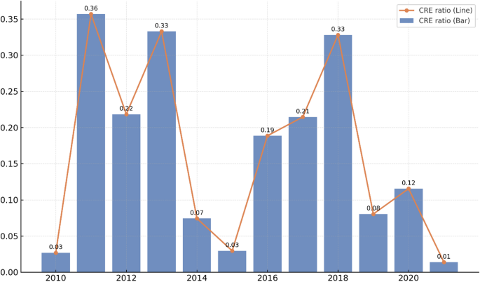
Temporal trend of the average CRE in Chinese prefecture-level cities.
In terms of the spatial pattern of CRE, Fig. 3 illustrates the dynamic changes in the CRE levels of Chinese prefecture-level cities from 2010 to 2021 using a color gradient ranging from dark green to dark blue. The levels are categorized as negative rebound (< 0), partial rebound (0–1), mild backfire (1–2), moderate backfire (2–5), and severe backfire (> 5)74,75. In 2010, the negative rebound effects were prominent in traditional industrial cities in Northeast China, such as Qinhuangdao (−1.868) and Handan (−1.174), due to post-crisis demand contraction in steel and chemical sectors, which led to a passive reduction in carbon emissions. From 2013 to 2015, partial rebound effects emerged in central and western cities like Chengdu (−1.276) and Chongqing (0.375), where the introduction of energy-saving equipment coincided with industrial expansion, causing emissions to grow more slowly than economic output. Between 2015 and 2018, coastal high-tech zones experienced mild backfire effects. Cities like Shenzhen (−1.735 → 0.331) and Dongguan (1.178) saw emissions increase to more than 1.5 times the expected reductions, mainly due to reliance on traditional power grids by data centers and similar industries. From 2018 to 2021, resource-based cities showed moderate backfire effects. For instance, in Lüliang (0.062), expansion of coal chemical capacity combined with low coverage of clean technology led to emission growth that exceeded expected reductions by 3.2 times. Special cases of severe backfire effects include Zhangzhou (2010: 8.662) and Fushun (2012: 32.671), where carbon emissions surged due to the relocation of high-energy industries or commissioning of petrochemical projects.
From a spatial evolutionary perspective, a core-periphery gradient shift is observed. Core cities in the Yangtze River Delta maintained low CRE through upgrading of the service sector, while surrounding cities that received relocated industries experienced CRE peaks. Geographic constraints and policy interventions also played significant roles. For example, Lijiang in the mountainous Southwest reduced CRE through hydropower development, while Yichun in the Northeast maintained stable levels through forestry transformation. In post-disaster reconstruction cases, such as Quanzhou in Fujian, the use of green building materials helped avoid a severe backfire, indicating the effectiveness of policy measures.
Figure 3 shows pronounced regional disparities. Economically developed areas sustained low CRE through technological upgrading, while resource-dependent cities and cities receiving industrial relocation faced more serious rebound effects. In terms of temporal dynamics, the national average CRE declined from 0.187 in 2010 to 0.115 in 2021. However, coal-dependent cities in Shanxi and Inner Mongolia remain a key challenge for emission reduction. Therefore, stronger regional coordination mechanisms are needed, alongside capacity constraints and clean technology subsidies targeted at cities with high backfire effects.

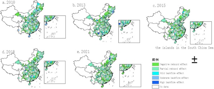
Spatial variation of carbon rebound effects in Chinese prefecture-level cities, 2010–2021. Map created using ArcGIS 10.8 ( based on the standard map service provided by the Ministry of Natural Resources of China, Map No. GS(2020)3184.
Results of factor analysis
Selection of driving factors and pearson correlation matrix
Based on the TOE framework, this study systematically constructs a framework for analyzing the factors influencing CRE across three dimensions: technology, organization, and environment. Thirty-eight explanatory variables are selected to explore the core drivers of CRE (Table 3).The technological dimension focuses on clean energy, digital technology, and the energy structure:① Clean energy technology is measured by the total number of green patent applications, including invention and utility model patents, reflecting the level of technological innovation and commercialization potential;② Digital technology is assessed through indicators of industrial development (e.g., fiber optic cable density, internet port availability, and employment share in the digital economy) and the digital economy index, quantifying its dual role in optimizing energy efficiency and enabling scale expansion;③ Energy structure is measured using energy consumption intensity as the core indicator, reflecting efficiency in energy utilization.The organizational dimension covers enterprises, government, and citizens:① Enterprises are assessed by their ESG scores, reflecting their capacity for low-carbon transformation;② Government actions are captured through indicators such as fiscal investment, financial decentralization, and environmental regulation, illustrating the effects of policy tools;③ Citizens’ environmental awareness is measured using indicators of environmental pollution and smog-related online search trends, reflecting public engagement.The environmental dimension integrates multidimensional factors from nature, the economy, society, and industry:① The natural environment includes extreme weather events and land use types (e.g., farmland and forest proportions);② The economic environment encompasses per capita disposable income, financial agglomeration, and the level of openness to trade;③ The social environment is assessed through factors such as population size and urbanization rate, reflecting demand-side pressure;④ The industrial structure is characterized by two core indicators: the industrial upgrading index (weighted by the value-added share) and sophistication level (measured by the tertiary-to-secondary sector ratio).
To identify and eliminate multicollinear variables and avoid information redundancy or interpretive bias during model fitting, a systematic Pearson correlation analysis was conducted for all candidate features (see Fig. 3). The results indicate that some variables are highly correlated (|r| > 0.8)76, such as GPA and GIA; GU Pat; GDI and DEI or EI; and UIS1 and UIS2. Variables with overlapping definitions or similar constructs (e.g., OFD, PBAP, cropland, UL) were removed. In contrast, certain variable pairs with high correlation but distinct interpretive value within the CRE mechanism—such as GPA and GIA, or GDI and EI—were retained for further analysis in the mechanism modeling phase. This approach reduces the risk of multicollinearity while preserving the theoretical and empirical dimensions necessary for interpretation, thus improving model robustness and explanatory power (Fig. 4).

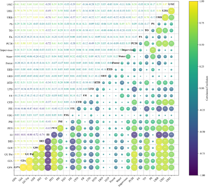
Pearson correlation matrix.
Key factor identification
① Multiple Regression Results from the Panel Regression Model.
To more accurately analyze the influencing factors of CRE, this study employs a panel regression model. Panel regression effectively addresses individual heterogeneity and time-series characteristics in panel data, thereby improving the accuracy and reliability of the estimates. For clarity, five key variables were selected. Table 4 reports the multiple linear regression results. The following variables have a positive effect on CRE: ER, HTD, and water. The following variables have a negative effect on CRE: DEI and UIS2.
② Model Selection and Validation.
Nine commonly used machine learning algorithms were trained on the dataset. Grid search was used for hyperparameter optimization to improve model performance and generalization. To avoid overfitting on a single training set, five-fold cross-validation was applied. Model performance was evaluated using root mean square error (RMSE), mean absolute percentage error (MAPE), and the coefficient of determination (R2). Figure 5 presents the results for each algorithm.

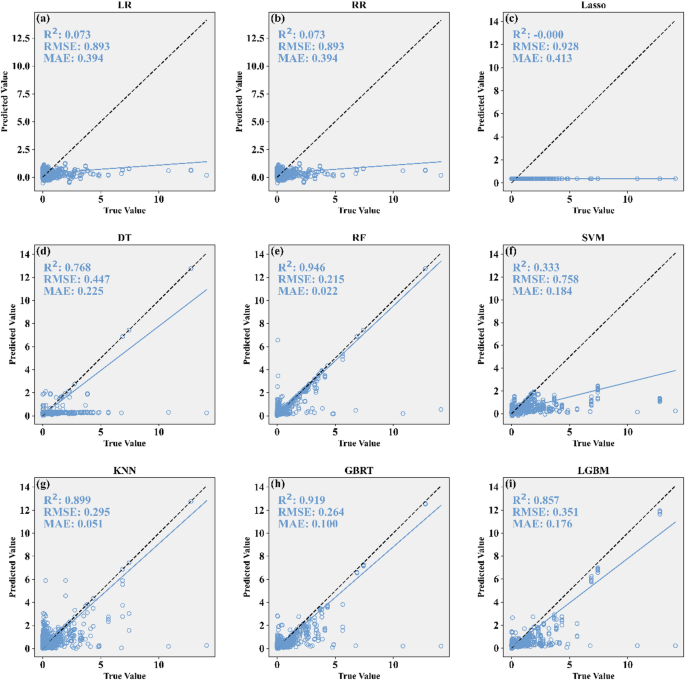
Model fitting results for each algorithm. (a) Linear regression (LR); (b) Ridge regression (RR); (c) Lasso regression; (d) Decision tree (DT); (e) Random forest (RF); (f) Support vector machine (SVM); (g) K-Nearest Neighbors (KNN); (h) XGBoost (XGBT); (i) LightGBM (LGBM).
In the context of regression analysis, lower RMSE and MAE values indicate higher predictive accuracy, while an R2 value closer to 1 reflects better model fit77. As shown in Fig. 5, the RF model achieved the highest predictive performance among all evaluated algorithms, with an R2 of 0.946, a very low RMSE of 0.215, and an MAE of just 0.022. Compared with other models, such as GBRT (R2 = 0.919), KNN (R2 = 0.899), and LGBM (R2 = 0.857), RF demonstrated superior accuracy and stability. These results suggest that the random forest model provides the most reliable and precise fit for predicting CRE in this study. Therefore, the RF algorithm is selected for the subsequent feature importance analysis, with GBRT used as a complementary method to identify and quantify the key drivers of CRE.
③Ranking of Feature Importance.
To further examine how different features influence the CRE, this study employs the SHAP method to measure and compare the predictive power of each variable. Results from both the GBRT and Random Forest models indicate that the top ten most important features consistently include DEI, the number of HTD, ER, Water, and UIS2. These features exhibit the strongest predictive performance for CRE. Moreover, Table 5 shows that these five features are ranked similarly across both models, supporting the robustness of the findings. These results not only validate previous studies but also provide new insights. Traditional econometric approaches often struggle to compare the relative importance of variables due to issues such as differing units and model specifications. The SHAP method addresses this limitation effectively.
④Main Feature Variables and Their Predictive Patterns for CRE.
Based on the SHAP results from the GBRT and Random Forest models, we selected key features such as DEI, the number of HTD, ER, Water, and UIS2 for ALE visualization.
Figure 6 presents ALE plots illustrating the effects of these features on CRE. These plots reveal nonlinear impacts and key thresholds. The DEI shows a bidirectional effect on CRE. When the DEI is below 0.3, insufficient digital penetration increases CRE. When it exceeds 0.6, smart algorithms help mitigate the CRE. In northern regions, where HTD exceeds 15 days, carbon release from permafrost and increased heating demand contribute to a nonlinear rise in CRE. When HTD surpasses 40 days, this trend may trigger carbon lock-in effects in energy systems. The effect of ER is stage-dependent. Low intensity (ER < 80) promotes investment in emission-reduction technologies. High intensity (ER > 90) may reduce marginal returns due to rising compliance costs. Water bodies serve as carbon sinks. A moderate share (5%–15%) helps reduce CRE. However, excessive expansion (i.e., over 15%) weakens this mitigating effect. A higher share of services (UIS2 > 3.0) reduces emissions from energy-intensive industries. Yet, during the transition phase (i.e., UIS2 = 1.5–3.0), carbon leakage may occur due to industrial relocation.

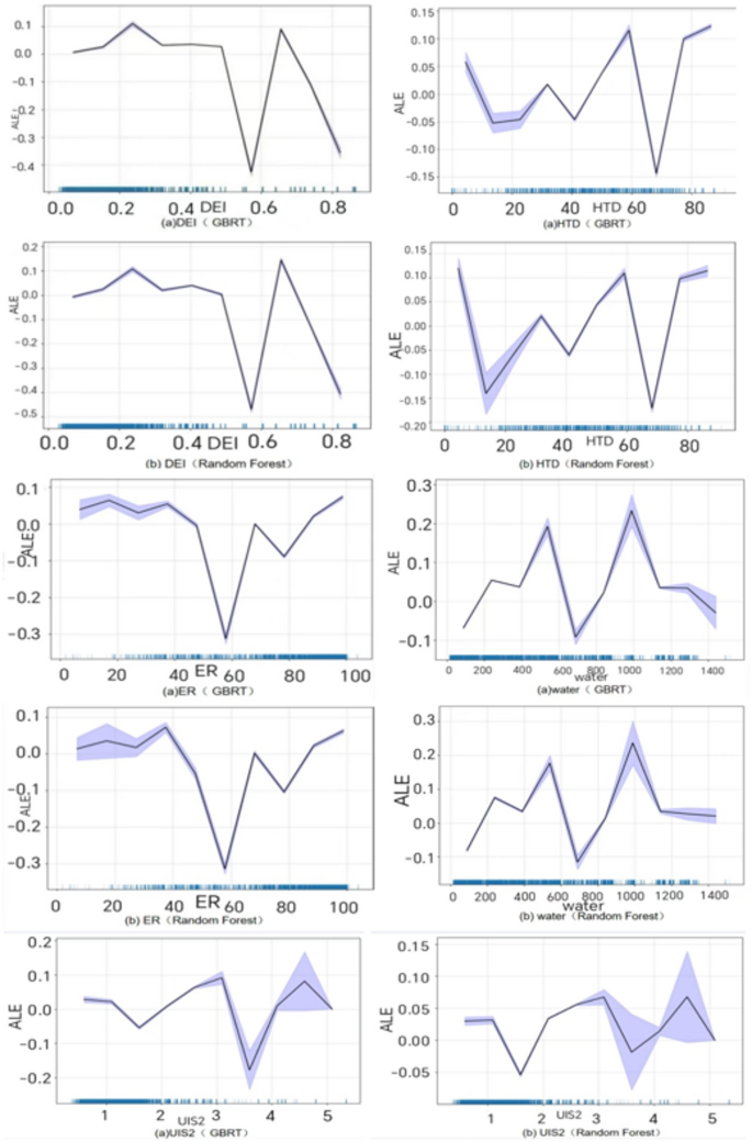
ALE plots of key factors and their effects on CRE.
Discussion
Discussion on the spatiotemporal distribution of CRE
Based on a detailed analysis of temporal trends, this study finds a dynamic offset between emission reductions driven by intensity decline and increases driven by economic growth. This offset follows a downward but fluctuating trend. Compared with the findings of Wu et al. (2018), the CRE patterns identified in this study are more stable overall but also exhibit greater short-term volatility.From a spatial perspective, the distribution of CRE varies significantly over time across urban agglomerations. Some cities exhibit weak or strong rebound effects, while others show no rebound or even suppressive effects. The relationship between efficiency gains and CRE is not uniform across regions. External shocks, such as the COVID-19 pandemic in 2020, caused deviations in the carbon intensity trend. These disruptions led to substantial heterogeneity in the eventual rebound effects across urban clusters, further highlighting the complexity of CRE.Future research should investigate how regional differences in industrial structure, energy consumption, and growth models influence the spatiotemporal patterns of CRE. This would help deepen our understanding of how regional economic characteristics shape CRE outcomes. Comparative studies across regions should also explore intra-urban cluster variation and its underlying drivers. These insights can support the development of more targeted regional emission reduction policies.In addition, long-term tracking of external shocks is needed to evaluate both the short- and long-term impacts of such disruptions on CRE. This would help improve policy responses to uncertainty. However, while this study identifies the spatiotemporal features of CRE, it does not fully explain the underlying mechanisms. It lacks a systematic analysis of interregional interactions and feedback effects. Moreover, the external shock analysis mainly focuses on the 2020 pandemic. Future research should expand to include a broader range of case studies to better assess the effects of various unexpected events on CRE.
Discussion on the drivers of CRE
This study uses machine learning models to explore the relationship between efficiency improvements and CRE, indicating a potential decoupling between the two. DEI, HTD, ER, Water, and UIS2 are identified as the main drivers of CRE. These factors show significant threshold effects. Compared to traditional regression models, machine learning techniques such as Random Forest and XGBoost better capture nonlinear relationships among variables. These models uncover the complex mechanisms of key drivers and offer more precise tools for dynamic CRE analysis.
Future research can be extended in the following directions: First, it is important to deepen the analysis of the pathways and mechanisms through which core variables—particularly DEI and ER—affect CRE. This includes clarifying both direct and indirect effects, as well as examining heterogeneous impacts across different regions and industrial contexts to support more targeted regional emission reduction strategies.Second, based on the threshold features identified by machine learning, future studies could explore how the marginal effects of drivers on CRE vary across different threshold intervals. This would help identify ways to optimize variable configurations through policy adjustments to mitigate CRE.Third, the combination of modeling approaches could be expanded by exploring the applicability of various machine learning algorithms (e.g., LSTM, CatBoost) in CRE analysis. It is also worth considering the integration of these models with causal inference methods (e.g., structural equation models, causal forests) to enhance both explanatory power and policy relevance.
Moreover, although this study identifies key variables, some potential influencing factors may still be omitted. Future research should appropriately expand the set of variables to include socio-economic factors such as financial agglomeration, trade openness, and urbanization level. This would allow for a systematic assessment of their roles in the CRE formation mechanism. Notably, CRE exhibits significant variation across regions. Future studies could establish a multi-regional comparative analysis framework to explore the causes of regional differences and carbon emission transfer pathways, thereby revealing the potential and constraints for coordinated regional emission reductions.
Finally, to promote more comprehensive research development, it is recommended to further analyze the interactions between CRE and other environmental or socio-economic variables, such as air quality, economic development, and social equity. This would provide empirical support for the formulation of multi-objective environmental governance policies. In terms of research design, a machine learning-based CRE prediction system could be developed. Combined with simulation techniques, this system would evaluate the effects of regional emission reduction policies and support local governments in achieving more scientific, dynamic, and precise carbon management.
Limitations and future research
This study has several limitations that should be acknowledged. First, the analysis is based on data from Chinese prefecture-level cities between 2010 and 2021, which may not fully capture longer-term trends or recent structural shifts in energy and digital policy. Second, while machine learning models offer strong predictive performance, they remain inherently correlational and do not establish causal relationships. Although interpretability tools (SHAP and ALE) are employed to illuminate variable contributions, the mechanisms identified should be further validated through causal methods or experimental designs. Third, the variable selection, though grounded in the TOE framework, may not encompass all relevant factors—such as behavioral elements, international market fluctuations, or sub-city-level heterogeneity—that could influence CRE. Future research could extend this work by incorporating dynamic temporal modeling (e.g., LSTMs or transformer-based approaches), integrating more granular data, or applying causal machine learning techniques to better identify policy-sensitive pathways.
link